Chapter 4 Exploratory Data Analysis (EDA)
Initial notes developed by Thumbi Mwangi1 and Jonathan Dushoff2 for the MMED course 2019
1 Centre for Epidemiological Modelling and Analaysis, University of Nairobi
2 McMaster University, Canada
It entails analyzing and visualizing data in order to better understand your dataset.
EDA involves several steps:
- Importing the data
- Cleaning the data
- Processing/manipulating the data
- Visualising the data
The first three often take the most time (>80%), and this is mainly because researchers undervalue them.
There’s never time to do it right … but there’s always time to do it over!
4.1 Tools for exploratory data analysis
library(tidyverse)
# loads packages tidyr; dplyr; ggplot2; readr; purrr; tibble; stringr; forcats; lubridate; haven
Tidyverse is a collection of R packages that are designed for explotory data analysis. The packages include:
 library(tidyr)- Helps you to organise data (tidy data). It has some functions such as:
- pivot_longer(): converts data to a long format
- pivot_wider(): converts data to a wide format
- separate(): splits a single column into multiple columns
- unite(): combine multiple columns into a single column
 library(dplyr)- Helps in data manipulation (grammar of data manipulation). It includes functions such as:
- select(): picks columns (or variables) using their names
- filter(): picks rows based on their values
- group_by(): perform operations (e.g addition, subtraction) using groups
- summarise(): summarise the dataset based on selected operations
- arrange(): orders the rows
- full_join(): merges two datasets using unique identifiers
- mutate(): adds new columns or manipulates existing columns
 library(readr)- Provides an easier way of importing data into R. It includes functions such as:
- read_csv(): importing files with comma separated values(CSV)
- read_csv2(): importing files with semi-colon delimited values
- read_delim(): importing files with any delimiter
- read_fwf(): importing files with any fixed width
- read_tsv(): importing files with tab separated values
- read_table: importing files with whitespace-separated values
 library(tibble)- It is a “lazy” form of the dataframe and makes it easier to use large datasets.
 library(forcats)- It provides functions for changing order of factors or the values. Some of the functions include:
- fct_reorder: Reorders a factor using another variable
- fct_relevel: It reorders the order of factors
 library(stringr)- Allows you to easily manipulate strings. It includes functions such as:
- str_subset(): extracts matching components in a string
- str_replace(): replaces the matches with a new text in a string
- str_to_lower(): converts a string to lower case
- str_to_upper(): converts a string to upper case
- str_to_title(): converts a string to title case
- str_to_sentence(): converts a string to sentence case
 library(purrr)- Allows you to work with loops. It includes functions such as:
- map(): allows malnupilative functions to be executed for loops and other vector changes
 library(ggplot2)- Allows you to visualise data. It includes functions such as:
- geom_col(): Used to visualise bar graphs
- geom_histogram(): Used to visualise histograms
- geom_sf(): Used to visualise simple features (shapefiles)
 library(lubridate). This package makes it easier for one to convert dates. some of the functions include:
- floor_date(): round down date to the nearest unit (months, weeks, years etc)
- epiyear(): convert years according to the epidemiological week calendars
- with_tz(): convert time to a specific timezone
Another important package which is not part of the tidyverse packages is the library(haven) which allows you to import data in foreign statistical formats. It includes functions such as:
- read_sas(): # read SAS files
- read_sav(): # read SPSS files
- read_dta(): # read Stata files
Kindly note that:
Variable: a measure (values) of the same attribute across observation units (eg weight, age, infection status)
- Variable = column
Observation: a unit e.g a person - and all the variable values associated with the unit
Observation = row
Observational unit forms a table
4.2 Pipes in R %>%
The pipe, %>% , from the package “magrittr” - and loaded automatically with library(tidyverse)
Helps write more readable code
4.3 Importing data
To learn on exploratory data analysis, we will use the datasets ideal1 and ideal2. As the data is in CSV format, we will import data using read_csv() function.
# Import the package to the R environment. This is usually
# done once per R session

library(tidyverse)
library(lubridate)

## Import the data into the R environment

ideal1 <- read_csv("https://raw.githubusercontent.com/ThumbiMwangi/R_sources/master/ideal1.csv")
ideal2 <- read_csv("https://raw.githubusercontent.com/ThumbiMwangi/R_sources/master/ideal2.csv")
Now let us have a glimpse of our imported data.
ideal1## # A tibble: 30 × 8
## CalfID CalfSex sublocation CADOB ReasonsLoss Education Distance_water
## <chr> <dbl> <chr> <chr> <dbl> <chr> <chr>
## 1 CA020610151 1 Karisa 3/11/2… NA Secondar… At household
## 2 CA020610152 1 Karisa 4/10/2… NA No forma… <1 km
## 3 CA010310064 1 Kokare 3/1/20… 7 Primary … <1 km
## 4 CA031310367 1 Yiro West 4/6/20… 7 Primary … 1-5 km
## 5 CA051910545 2 Bujwanga 7/4/20… NA Primary … <1 km
## 6 CA051810516 1 Luanda 11/3/2… NA Primary … <1 km
## 7 CA010210036 2 Kidera 12/3/2… 7 Primary … 1-5 km
## 8 CA052010596 2 Magombe East 2/9/20… NA No forma… 1-5 km
## 9 CA041610476 1 Ojwando B 4/9/20… NA Primary … <1 km
## 10 CA051910566 2 Bujwanga 5/9/20… NA No forma… <1 km
## # … with 20 more rows, and 1 more variable: RecruitWeight <dbl>We can observe that the data is imported as a tibble, and contains 30 observations (rows) and 8 variables (columns).
Also, it is important to note that tibble is regarded as a “lazy” dataframe because it only displays the number of rows that can fit on the console ( compare this with importing the data using read.csv() function).
ideal2## # A tibble: 270 × 9
## VisitID CalfID VisitDate Weight ManualPCV Theileria.spp. ELISA_mutans
## <chr> <chr> <chr> <dbl> <dbl> <dbl> <dbl>
## 1 VRC010151 CA020610151 9/11/2007 19 37 0 0
## 2 VRC010152 CA020610152 11/10/2007 23 35.8 0 0
## 3 VRC210545 CA051910545 1/9/2008 33 27 1 0
## 4 VRC110224 CA030810224 1/12/2008 33 44 0 0
## 5 VRC160223 CA030810223 1/12/2008 54 30 0 1
## 6 VRC110038 CA010210038 2/7/2008 25 26 0 0
## 7 VRC160036 CA010210036 2/7/2008 34 26 0 0
## 8 VRC060375 CA031310375 2/12/2008 19 43 1 0
## 9 VRC210151 CA020610151 3/4/2008 39 40 0 0
## 10 VRC260152 CA020610152 3/4/2008 71 40 0 0
## # … with 260 more rows, and 2 more variables: ELISA_parva <dbl>,
## # Q.Strongyle.eggs <dbl>The ideal2 dataset has 270 observations and 9 variables.
Next, we need to view the whole dataset.
# Type this in your console
View(ideal1)

View(ideal2)- We are able to observe that both datasets have a CalfID
- The calfsex and ReasonsLoss columns need to be recoded
- VisitDate is in a date format that R does not treat it as a date
- Five tests were done on the calves during different visits
4.4 Cleaning the data
We need to clean this data. We will:
4.4.1 Merge the dataset
As earlier mentioned, we merge data using a unique identifier(s) found in both datasets. In this case, it is the calf ID.
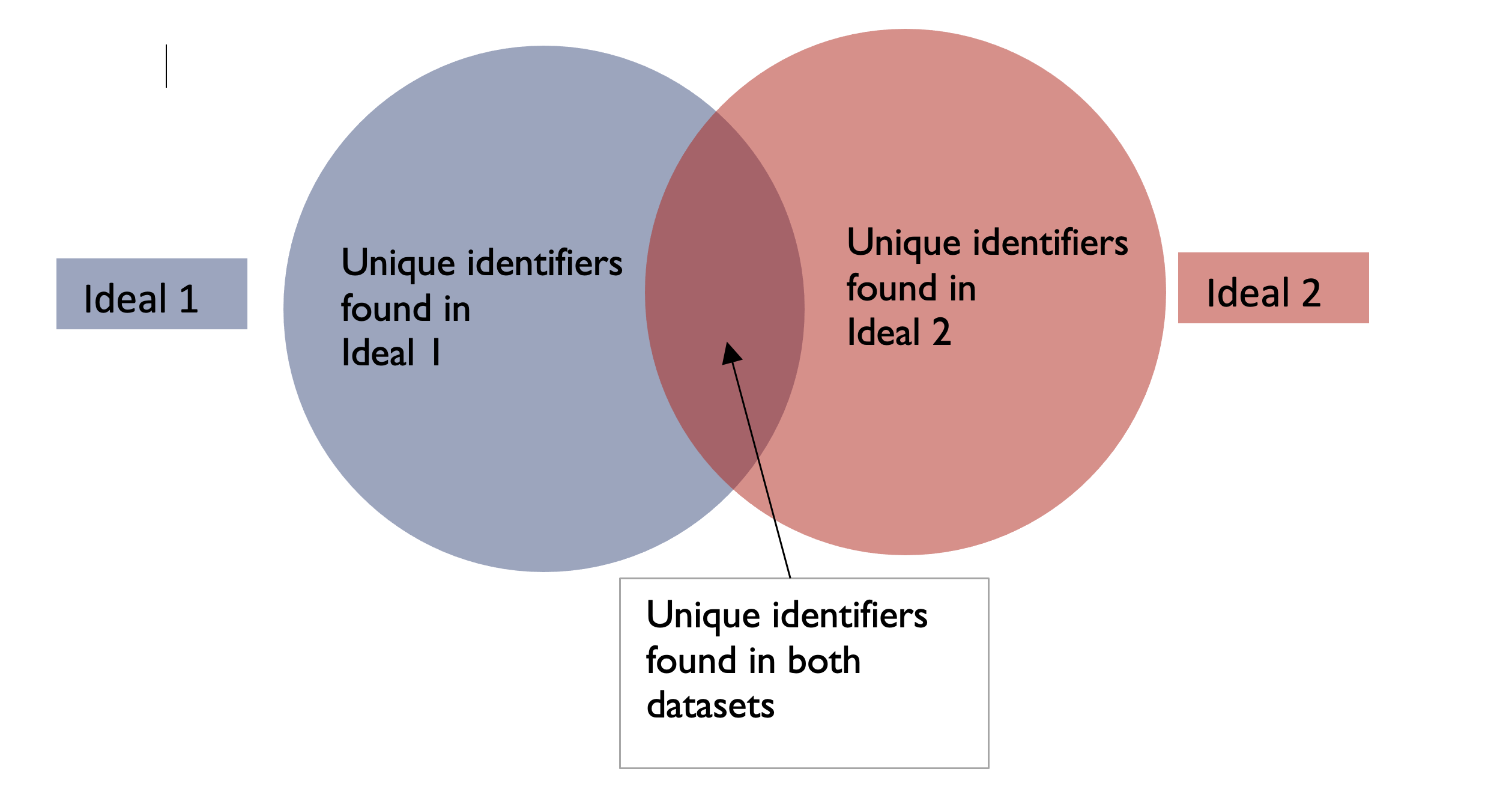
Unique identifiers may be found only in one of the datasets, or both
There are four types of merging data using tidyverse:
- Full join: combines the two datasets into one, regardless of whether the unique identifier(s) are found in both datasets
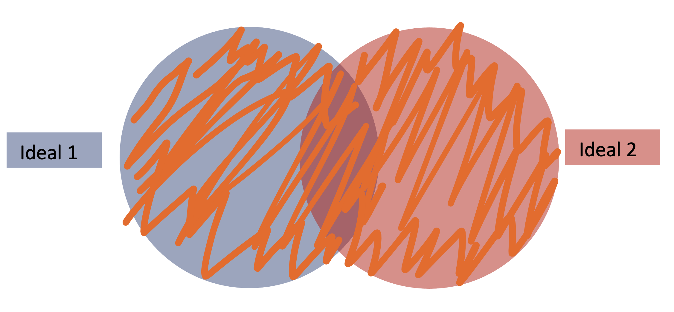
Full join combines the two datasets, regardless of whether a unique identifier is not found in both datasets
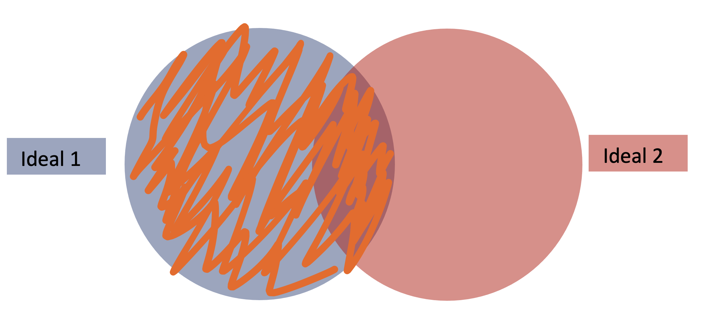
- Left join: combines the two datasets using the unique identifiers of the dataset on the left. If a unique identifier is only found on the right dataset but not on the left, then it will not be included.
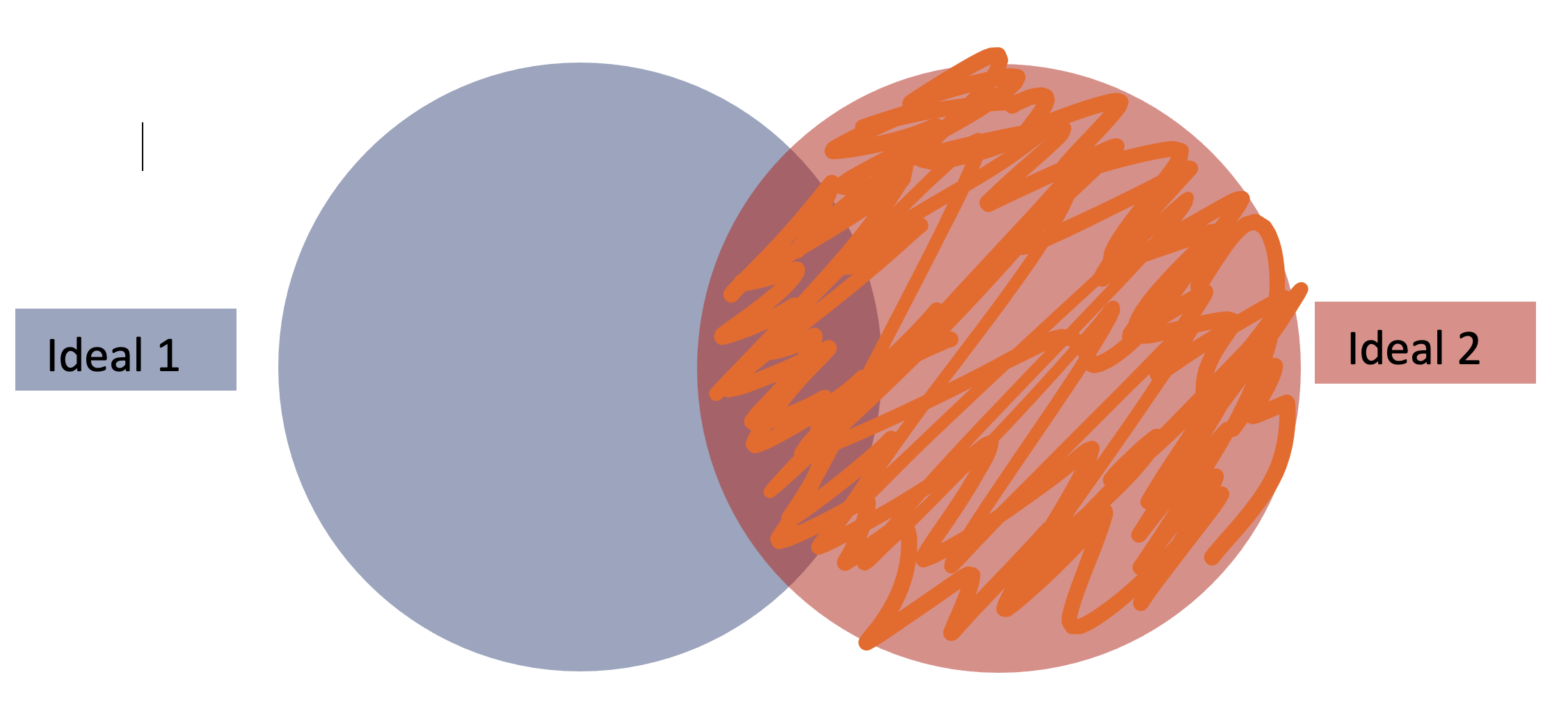
 c) Right join: combines the two datasets using only the unique identifiers of the dataset on the right. If a unique identifier is only found on the left dataset but not on the right, then it will not be included.
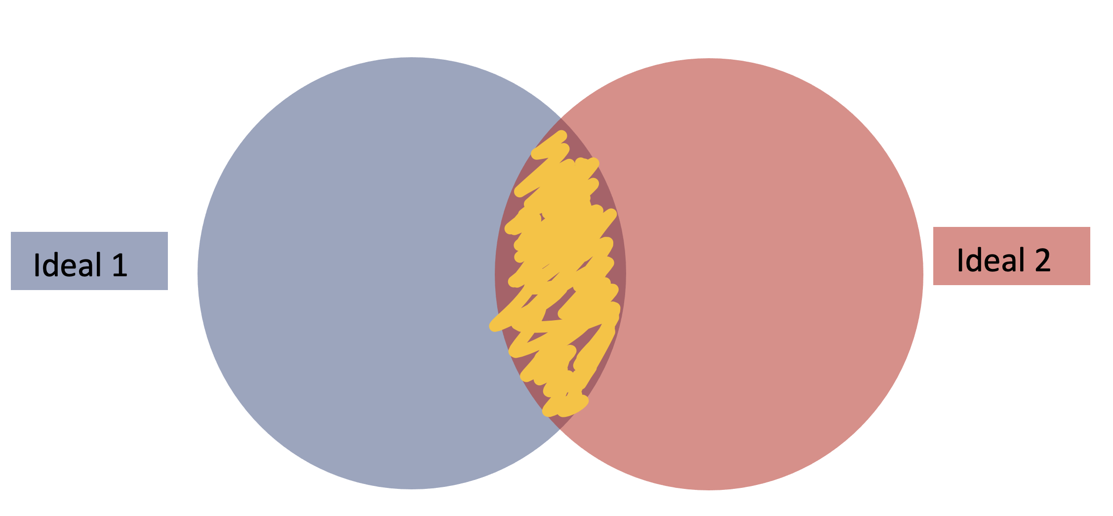
 d) Inner join: combines the two datasets using only the unique identifiers found in both the right and left datasets. If a unique identifier is only found on one of the datasets, then it will not be included.
 Let us now join our data using full_join()
##merge the dataset
# The dataset you call first is treated as the dataset on the left

ideal3 <- ideal1%>%
  full_join(ideal2, by="CalfID")

## Or, you can also write the code as below

ideal3 <- full_join(ideal1, ideal2, by="CalfID")
Our merged dataset has 270 observations and 16 variables (combining the columns on the first and second dataset).
Next, we will recode the dataset and clean the dates to a format that R understands
4.4.2 Data wrangling
# We will do the following:
##- recode the Calfsex from 1/2 to Male/Female, using the recode funtion
##- recode the ReasonsLoss variable
##- change the date format of the calf date of birth (CADOB) and VisitDate

ideal3a <- ideal3%>%
  mutate(CalfSex=recode(CalfSex, "1"="Male", "2"="Female"))%>%
  mutate(ReasonsLoss=recode(ReasonsLoss, "6"="Sold", "7"="Death", "12"="Owner Refusal", "18"="Relocation"))%>%
  mutate(CADOB=dmy(CADOB))%>% # here, you may also use the base R function, as.Date()
  mutate(VisitDate=dmy(VisitDate))
Our data is now in a better format, with dates that are understood by R, and also recoded data for the factors.
We will now try to extract the visit number from the VisitID.
head(ideal3a$VisitID)## [1] "VRC010151" "VRC210151" "VRC260151" "VRC310151" "VRC360151" "VRC060151"- Looking at data from this column, we observe that the ID has 9 characters, where the 4 and 5 character has the visit number. We will extract this column using the str_sub() function
# We extract the visit number from the Visit ID using str_sub() function

ideal3a <- ideal3a%>%
mutate(visit_number=str_sub(VisitID, 4, 5))- Finally, we will change the columns on the tests conducted on the calves into a long format. To do this, we will use the pivot_longer() function.
4.4.3 pivot_longer()
-Briefly, this function gathers multiple columns into key-value pairs. We need to tell the function which columns are to be converted to long format, and the new names of the two columns we will create (one column contains the previous column name, and the second column contains the values).
ideal3b<- ideal3a%>%
pivot_longer(c(ManualPCV, Theileria.spp., ELISA_mutans, ELISA_parva, Q.Strongyle.eggs), names_to="disease_type", values_to = "disease_values")- arrange() orders rows of a data frame by the values of selected columns.
## arrange our data by visit date

ideal3b<- ideal3b%>%
  arrange(VisitDate)
4.4.4 Grouping data
Grouping helps you to carry out different processes on grouped data. To do this, you first group the data (using group_by() function), carry out the process, then ungroup the data (using ungroup() function).
It is always a good practise to ungroup your data as you may forget and group the data in another section, ending up with wrong results as you will have created groups within existing groups.
Here, we can use the group_by() function to summarise the data where we would like to find out how many visits were done per sublocation
** Remember, as the meaning of the word, summarise() function summarises the dataset so it is a good idea to create a different object for the summarised data.
summarise_sublocation<- ideal3b%>%
  group_by(sublocation, visit_number)%>%
  summarise(count=n())


summarise_sublocation
## # A tibble: 141 × 3
## # Groups: sublocation [14]
## sublocation visit_number count
## <chr> <chr> <int>
## 1 Bujwanga 01 20
## 2 Bujwanga 06 20
## 3 Bujwanga 11 15
## 4 Bujwanga 16 15
## 5 Bujwanga 21 15
## 6 Bujwanga 26 15
## 7 Bujwanga 31 15
## 8 Bujwanga 36 15
## 9 Bujwanga 41 15
## 10 Bujwanga 46 15
## # … with 131 more rows4.4.5 A sample data set
- We can also use a sample dataset for dogdemography shared with you to practice the tidyverse functions.
dogdemography <- read_csv("DogcohortDemographics.csv") # import the data
dim(dogdemography)
## [1] 1207 11head(dogdemography)## # A tibble: 6 × 11
## IntDate HousehldID VillageID HhMmbrs OwnDogs DgsOwnd AdltDgs Puppies DogDied
## <chr> <chr> <dbl> <dbl> <dbl> <dbl> <dbl> <dbl> <dbl>
## 1 1/30/17 13-172-2 13 4 0 0 0 0 0
## 2 1/30/17 2-87-7 2 6 0 0 0 0 0
## 3 1/30/17 49-1-1 49 1 0 0 0 0 0
## 4 1/30/17 13-224-3 13 9 1 1 1 0 0
## 5 1/30/17 2-109-5 2 3 0 0 0 0 0
## 6 1/30/17 67-9-2 67 11 0 0 0 0 0
## # … with 2 more variables: NumDd <dbl>, DogBite <dbl>## rename the variables for clarity
dogdemography <- dogdemography%>%rename(interviewDate = IntDate # format as date
, householdID = HousehldID # format as character
, villageID = VillageID # format as character
, householdMembers = HhMmbrs # format as integer
, ownDogs = OwnDogs # format as logical
, numDogsOwned = DgsOwnd # format as integer
, adultDogsOwned = AdltDgs # format as integer
, puppiesOwned = Puppies # format as integer
, dogDiedPastMonth = DogDied # format as logical
, numDogsDiedPastMonth = NumDd # format as integer
, dogBitesPastMonth = DogBite # format as logical
)4.5 summarise()
- It is used to sumamrise each group to fewer rows
dogdemograohy1<-dogdemography %>%
  group_by(villageID) %>%
  summarize(count = n())
4.6 filter() rows/observations with matching conditions
dogdemography2<-dogdemography%>%
  filter(adultDogsOwned+puppiesOwned == numDogsOwned)%>%
  select(householdID,adultDogsOwned,puppiesOwned,numDogsOwned)
4.7 distinct()
- It removes duplicates
dogdemography2a<-dogdemography%>%
  group_by(numDogsOwned,adultDogsOwned,puppiesOwned)%>%
  select(adultDogsOwned,puppiesOwned,numDogsOwned)%>%
distinct() dogbites<- dogdemography%>%
group_by(dogBitesPastMonth)%>%
summarize(count = n()) Play with your data
- Don’t touch the original data
- Make scripts and make sure that they are replicable
- Don’t be afraid to play, experiment, probe
- You want to like your data-manipulation tools, and get your data as clean as possible
Summary
Let the computer serve you
- Input in the form that you want to input
- Manage in the tidy form that is efficient and logical
- Output in the way you want to output
Be aggressive about exploring, questioning and cleaning
Use this link for more resources on data wrangling: - There are other options of joining data called left_join(), right_join(), inner_join()
Kindly read more about this here: https://www.rstudio.com/wp-content/uploads/2015/02/data-wrangling-cheatsheet.pdf