Chapter 5 Data visualisation
The ggplot2 package from the tidyverse packages is used for data visualisation. gg stands for grammar of graphics.
You can build every graph from the same 3 key components:
- a data set: you provide the raw data that you would like to visualise
- a coordinate system default - cartesian coordinate system (can flip, fix them, use polar coordinates, transform - eg “sqrt,” “log” etc)
- geom - the visual marks that represent your data points. It represents what you see - the points, the lines, paths, text, labels, boxplots, bars, rasters etc - the type of plot the layer contains - see ggplot2 cheat sheet
In addition, you can provide the other components:
Scales - to render the layers correctly (map the data to the graphical output) - mapping continuous variables
Faceting - help you drill-down into the data as subplots using one or more variables (similar to pivot charts in Excel)
Themes - control details of the display - eg fonts, color scheme, size - customization of the display
This package allows you to create elegant data visualisations (print quality graphics) - rather quickly with very “fine grain control”
5.1 Starting with ggplot
When using one variable that is continuous, the following geoms are relevant:
- geom_area()
- geom_density()
- geom_dotplot()
- geom_freqpoly()
- geom_histogram()
- geom_qq()
When visualising one variable that is discrete, geom_bar() is relevant
For two variables where both x and y is continuous, we use the following geoms:
- geom_jitter()
- geom_point()
- geom_quantile()
- geom_smooth()
For two variables where x is discrete and y is continuous, the following geoms are relevant:
- geom_col()
- geom_boxplot()
- geom_dotplot()
- geom_violin()
Where both variables are discrete, you use a geom_count()
More on the relevant geom to use can be accessed here
For the visualisation tutorial, we will use the ideal dataset previously used in this tutorial.
5.1.1 Bar graphs
They are used to make a comparison between different groups or track changes over time. Bar graphs are best used when measuring large changes over time.
In ggplot, the geom used to plot bar graphs is geom_bar() and geom_col()
5.1.1.1 geom_bar()
library(tidyverse)

ideal <- read_csv("https://raw.githubusercontent.com/ThumbiMwangi/R_sources/master/ideal3a.csv")

ggplot(data=ideal, aes(x=ReasonsLoss1)) +
  geom_bar()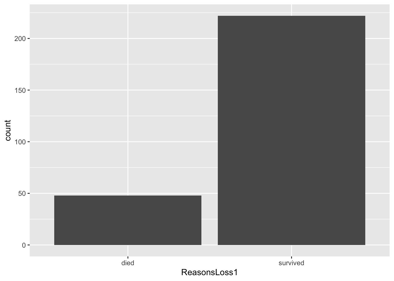
- We can see that our graph has a grey background and the labels of the x and y axis take the column names. We can customise our x and y axis labels and also add a title to our graph, as we change the background of the graph.
## Compare animals from the dataset that died and those that survived
ggplot(data=ideal, aes(x = ReasonsLoss1)) + # add the data
  geom_bar() + # choose the geom that you want to use to visualise your work
  theme_bw() + # background theme for your graphic. You can try changing the different themes to see the changes
  labs(x="", y ="Number of Calves", # renaming your x and y axis
       title = "Survival of calves in the first year of life") # adding a title to your graph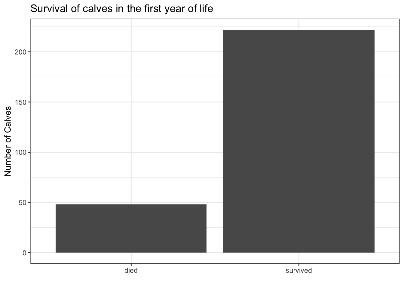
# Try change to the following themes
## theme_dark()
## theme_void()
## theme_classic()
From the above graph, we have used ggplot() to add the data together with the aesthetics, added the type of visualisation we wanted to use (geom_bar()) and the theme of our graphic. In addition, we have customised our x and y axis labels, and given a title to our graph.
Note that the geom_bar() only takes one variable. In our case, we have only included the x axis and it tabulated the frequencies and gave us a visualisation.
If you needed to plot a bar graph that takes in two variables, the x and y axis, you would use a geom_col()
5.1.1.2 geom_col()
- We will first summarise the ideal dataset and do a tally of how many calves were recruited in each sublocation.
calves_recruited<- ideal%>%
  select(sublocation)%>%
  group_by(sublocation)%>%
  dplyr::summarise(freq=n())

ggplot(calves_recruited, aes(x=sublocation, y=freq))+
  geom_col()+
  theme_bw()+
  labs(x="Frequency", y="Sublocation")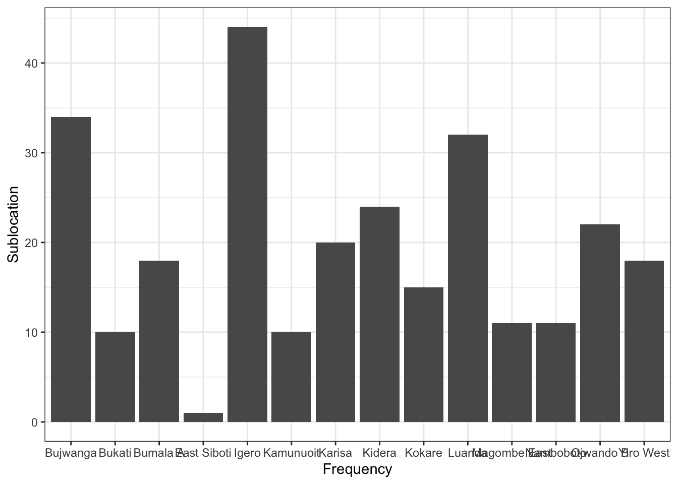
- When we look at our graph, it has given us the frequencies for each location and we were able to add the x and y axis. However, the sublocations in the x axis seem to be overlapping and so we can use the coordinate system, to flip our graph such that the x axis appears where the y axis is and vice versa
ggplot(calves_recruited, aes(x=sublocation, y=freq))+
  geom_col()+
  theme_bw()+
  labs(x="Frequency", y="Sublocation")+
  coord_flip() # flip our graph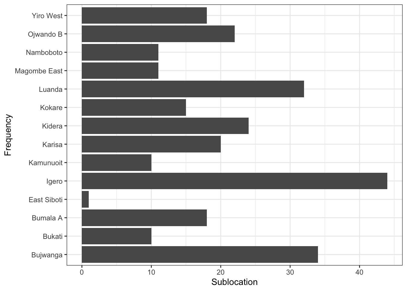
Much better! We are now able to read the sublocations pretty well. But it would make it easier if we were able to arrange the bars in descending order. We can use the reorder() function.
We will add this function in the x axis as we want to reorder out sublocations. Remember, the axis has been flipped so do not confuse the x and y axis.
ggplot(calves_recruited, aes(x=reorder(sublocation, freq), y=freq))+ # reorder function used here.
  geom_col()+
  theme_bw()+
  labs(x="Frequency", y="Sublocation")+
  coord_flip() # flip our graph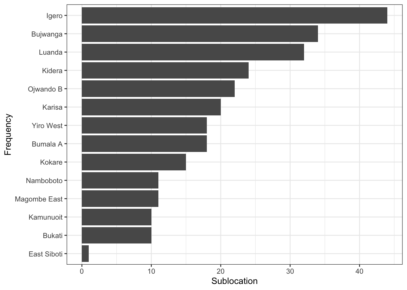
Now, let us say we wanted to know which calves were recruited in each sublocation, based on gender, and enable one to visualise that in the graphic.
We will first summarise our data based on how many calves were recruited in each village, based on gender.
calves_recruited1<- ideal%>%
  select(sublocation, CalfSex)%>%
  mutate(CalfSex=recode(CalfSex, "1"="Male", "2"="Female"))%>%
  group_by(sublocation, CalfSex)%>%
  dplyr::summarise(freq=n())

# visualise the data using a bar graph
ggplot(calves_recruited1, aes(x=reorder(sublocation,freq), y=freq, fill=CalfSex))+ # color the graph by sex
  geom_col()+
  theme_bw()+
  labs(x="Frequency", y="Sublocation")+
  coord_flip() # flip our graph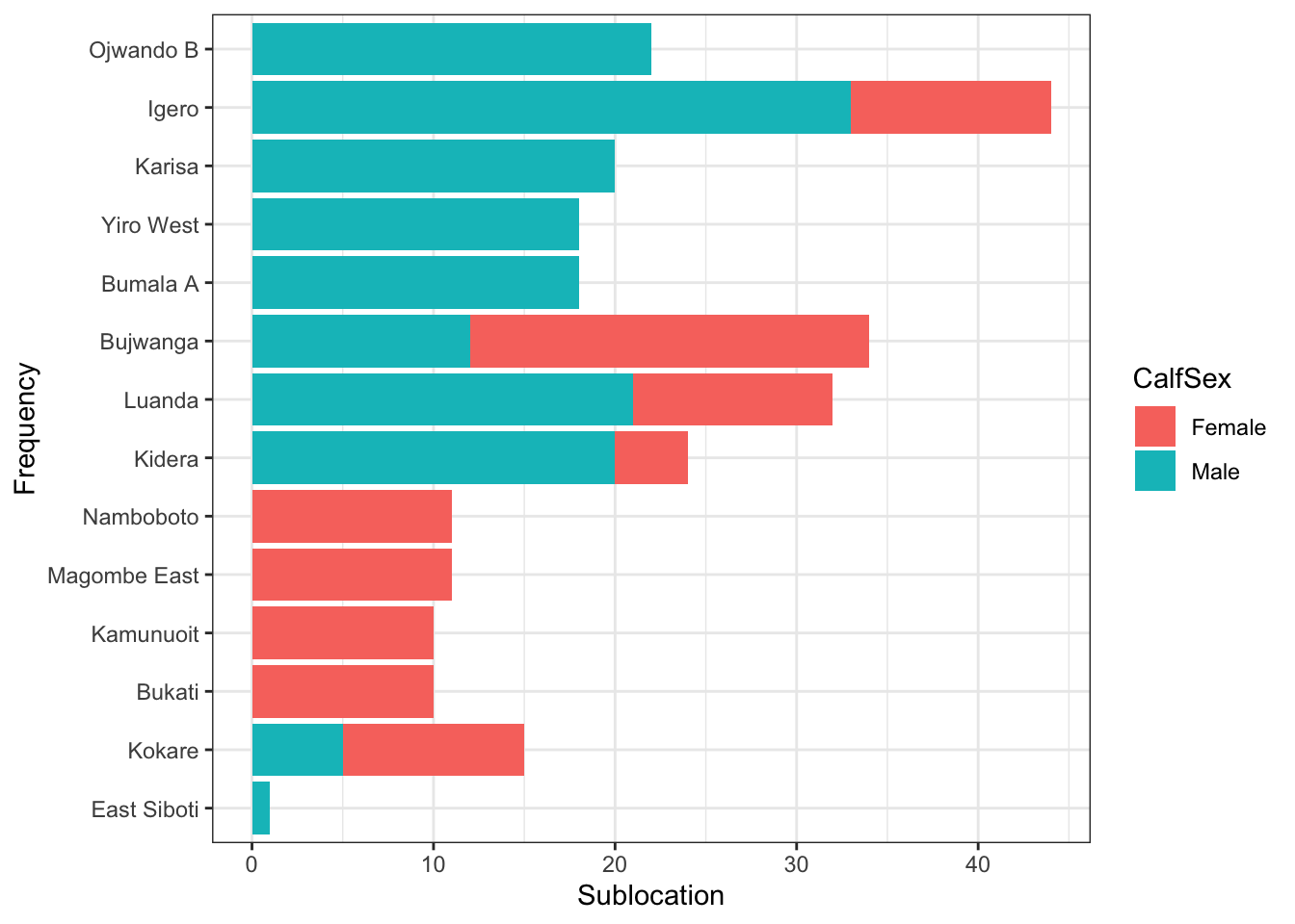
5.1.2 Line graphs
Like bar graphs, line graphs are also used to track changes over a time period. They can also be used to compare groups over time.
Line graphs require both x and y axis though both axis can only be a numeric variable (continuous or discrete) or a date.
To visualise this, we will use the visit date and calculate the average daily weight gain for the calves (using ADWG column).
# Survival by CalfSex - use color to add dimension of CalfSex
ideal_data <- ideal %>%
select(VisitDate1, ADWG)%>%
group_by(VisitDate1)%>%
mutate(ADWG1=mean(ADWG))%>%
ungroup()%>%
select(-ADWG)%>%
distinct()
ggplot(ideal_data, aes(x = VisitDate1, y=ADWG1)) +
geom_line()+theme_bw() # customise the x and y axis labels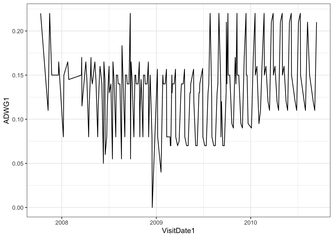 - The graph has shown us the trend over time, but it is diffult for us to understand the trend in the daily weight gain. Also, we would want shorter breaks in our x axis. In the next step, we will introduce the geom_smooth() graph
5.1.2.1 geom_smooth()
- As the name suggests, this graph “smoothens” the patterns in your data to aid the eye in seeing patterns. It used the generalised additive model if the observations are more than 1000 and changes to the loess smoothing method if they are less than 1000.
ggplot(ideal_data, aes(x = VisitDate1, y=ADWG1)) +
  geom_smooth()+theme_bw()+
  scale_x_date(date_breaks = "4 months", date_labels = "%b-%Y") # customise the x axis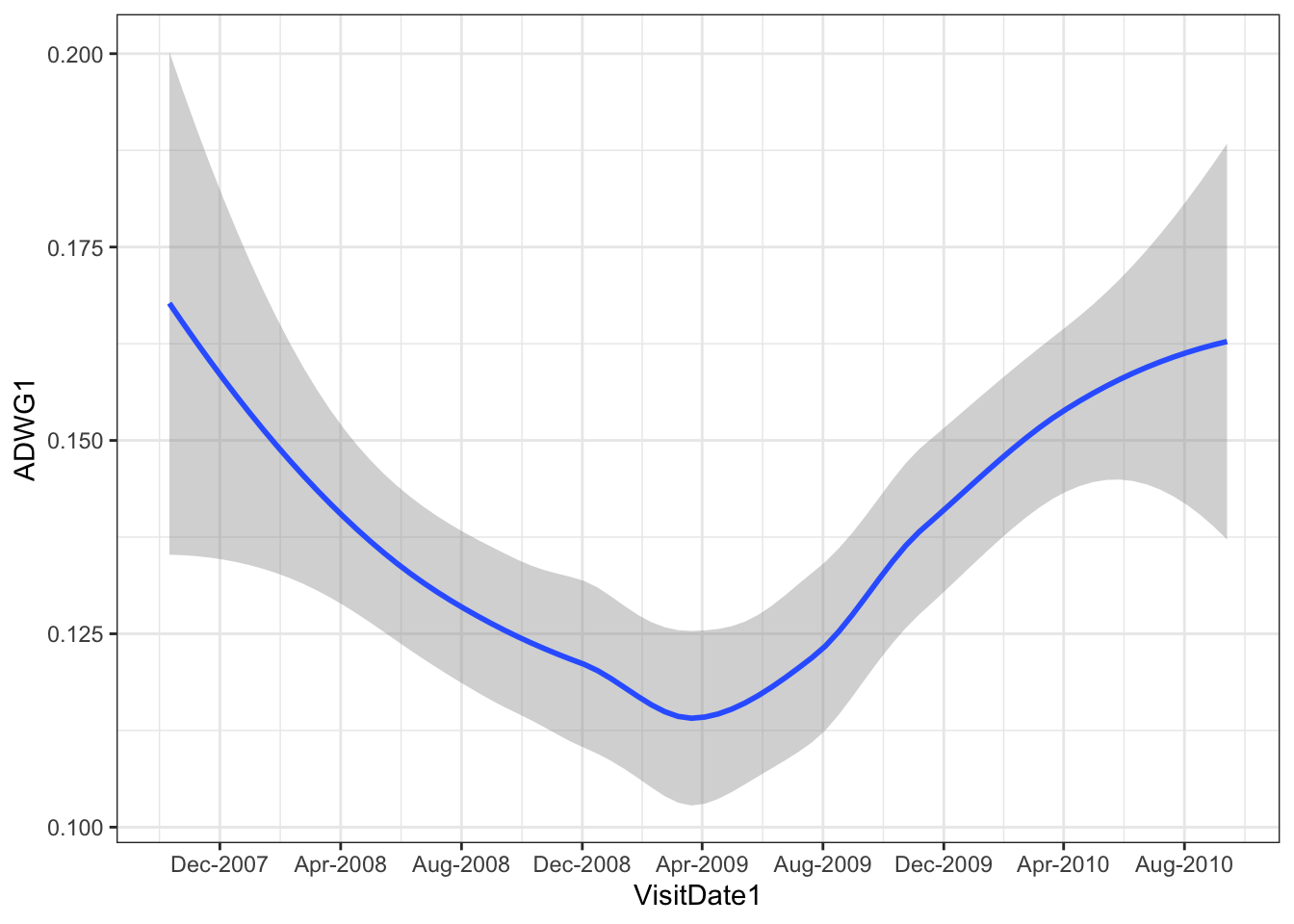
# customise the x and y axis labelsWe can now visualise the trend in the average weight gain of the calves. Similarly, we have customised the x axis to give us better date breaks and in an easy to read format. The grey ribbon represents the 95% confidence interval of the trend. You can change the smoothing of the graph by changing the span which is added in the geom_smooth().
In the above graph, try geom_smooth(span=0.2) and see how the visualisation of the graph changes.
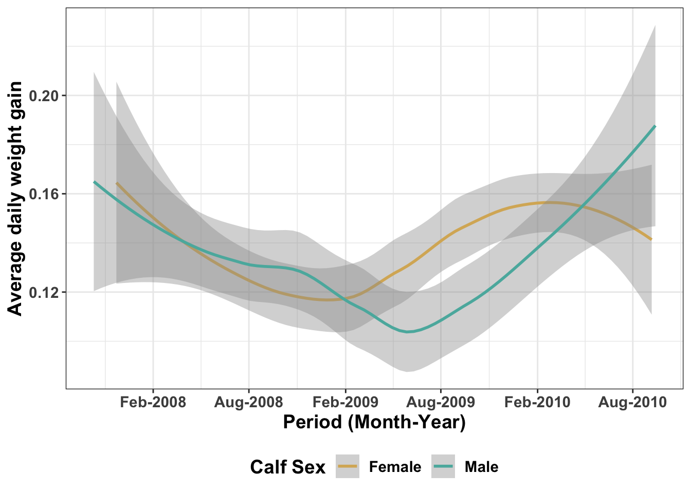
Suppose we wanted to compare the average weight gain of the calves based on sex, we can do this by first getting the average weight per visit date and visualising this.
ideal_data1 <- ideal %>%
select(VisitDate1, ADWG, CalfSex)%>%
mutate(CalfSex=recode(CalfSex, "1"="Male", "2"="Female"))%>%
group_by(VisitDate1, CalfSex)%>%
mutate(ADWG1=mean(ADWG))%>%
ungroup()%>%
select(-ADWG)%>%
distinct()
ggplot(ideal_data1, aes(x = VisitDate1, y=ADWG1, color=CalfSex)) +
geom_smooth()+theme_bw()+ scale_x_date(date_breaks = "4 months", date_labels = "%b-%Y")+
labs(x= "Period (Month-Year)", y="Average daily weight gain", color="Calf Sex")# color is used to change the title of the legend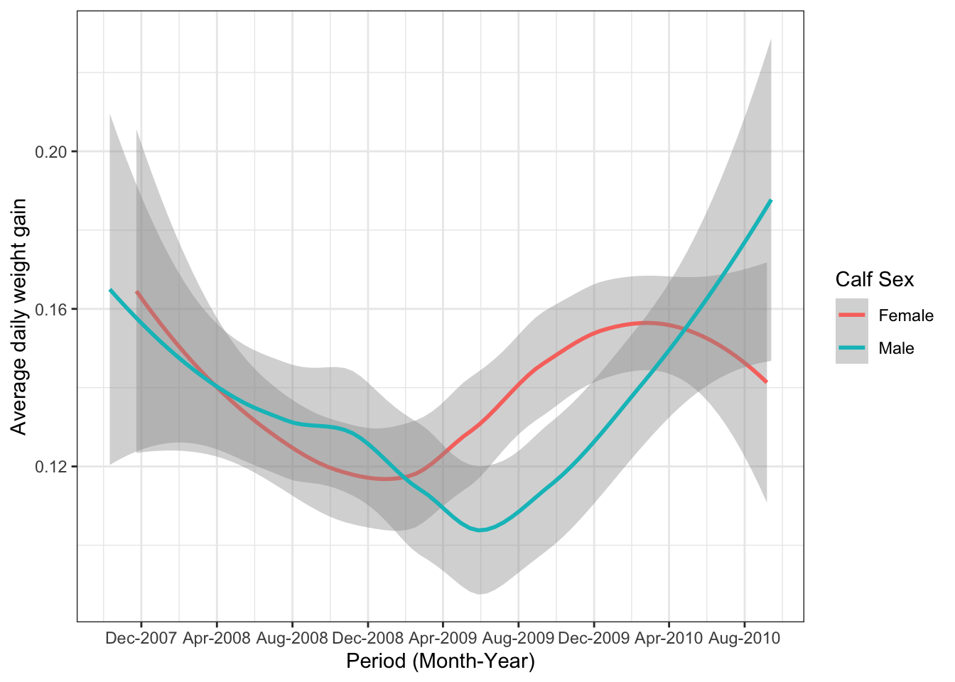 - We can now observe the trend in the average daily weight gain of the calves over a time period. We have also changed the title of the legend. It is important to note that the bar graphs use fill for color while line graphs use color. You can try change color to fill and see the difference in the graph above.
- If you used color in the aesthetics, then the title of the legend is changes using color and vice versa.
5.1.2.1.0.1 Faceting
Another interesting function in ggplot2 package is faceting which allows you to have two graphs in the same panel. If in the above graphic we wanted to have a separate line graph of male and female calves, we can use facet functions
facet_grid()
- It forms a matrix of panels defined by rows or columns.
ggplot(ideal_data1, aes(x = VisitDate1, y=ADWG1, color=CalfSex)) +
  geom_smooth()+theme_bw()+ scale_x_date(date_breaks = "6 months", date_labels = "%b-%Y")+
  labs(x= "Period (Month-Year)", y="Average daily weight gain", color="Calf Sex")+facet_grid(rows=vars(CalfSex))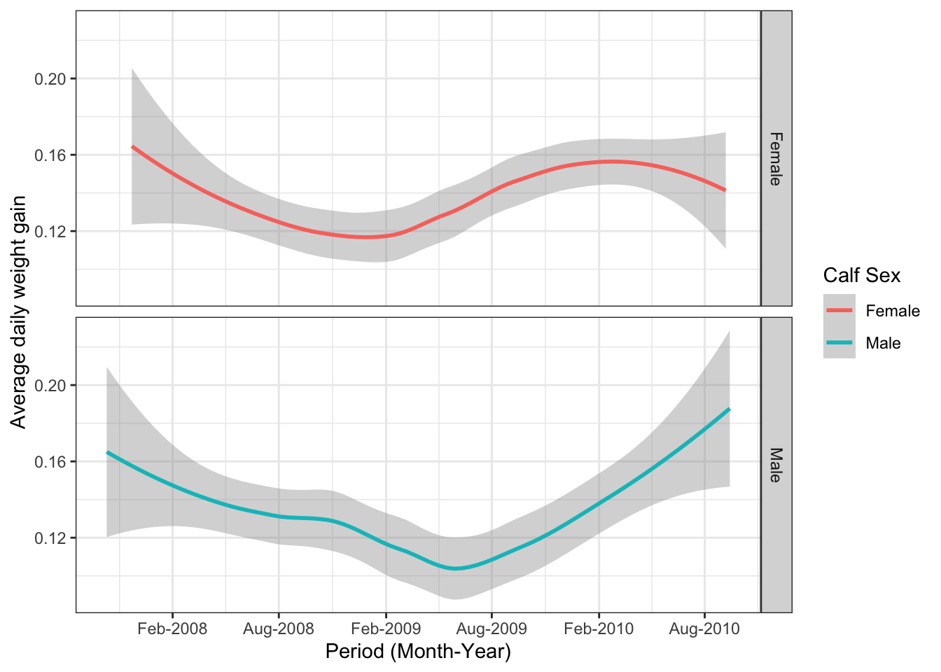
# replace facet_grid with facet_wrap and see how your graph looks like5.1.3 Histograms
- Similar to bar graphs, they are used to show distribution of variables. They usually take one variable and calculate the frequency, before visualising. The variable should be continuous or discrete.
5.1.3.1 geom_histogram
- We can visualise the packed cell volume of the calves (manualPCV column) in the ideal dataset.
ggplot(ideal, aes(ManualPCV)) + theme_bw() +
geom_histogram()+
labs() # customize the x and y axis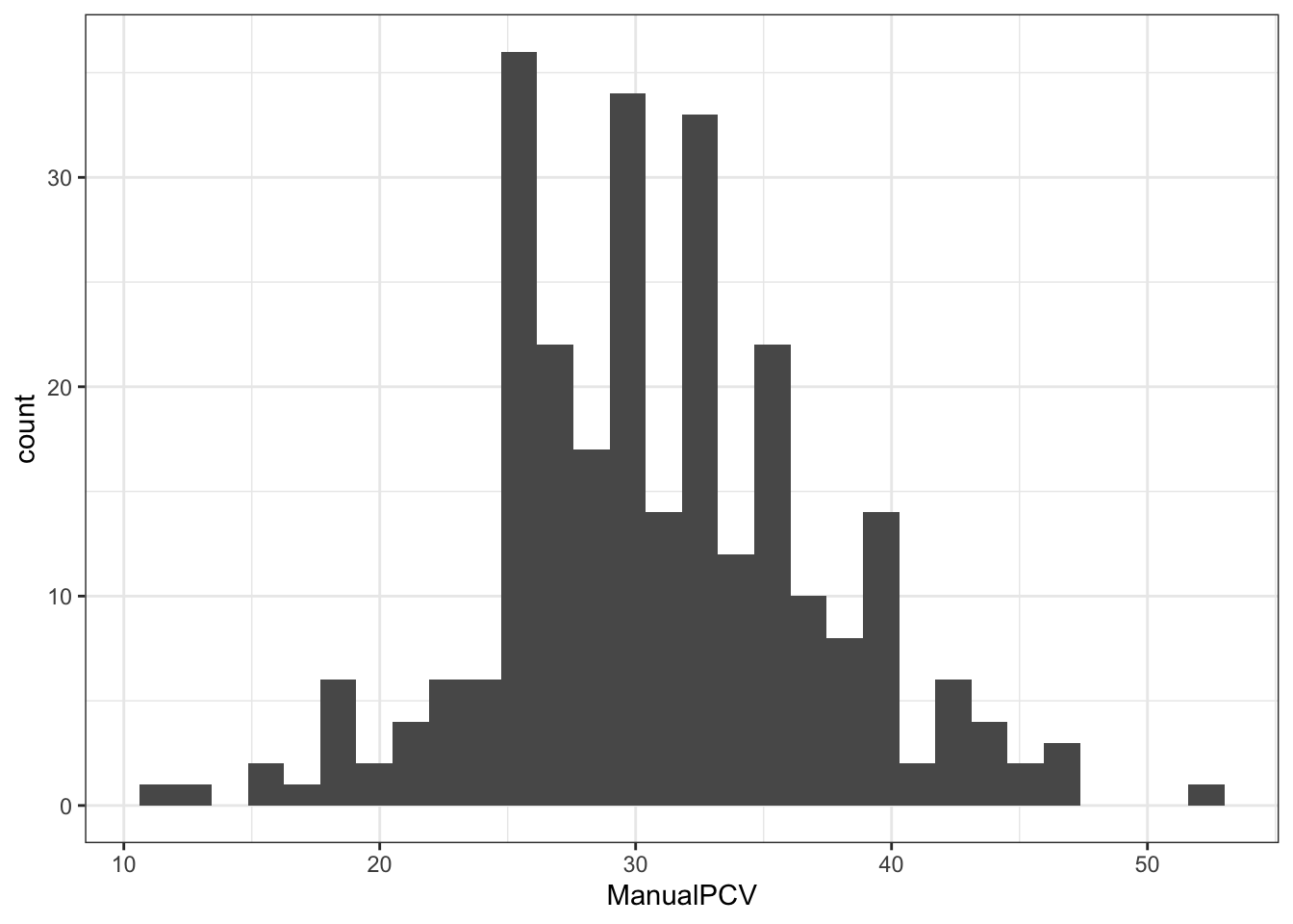 - You can change the range of values in your histogram by adding the bins By default, geom_histogram sets bins of 30, but this can change when you specify. Try this in your graph above and see how the visualisation changes geom_histogram(bins=20)
- We can even compare two variables in a histogram , as seen below
ggplot(ideal, aes(x = ManualPCV, fill=ReasonsLoss1)) + theme_bw() +
geom_histogram() + labs(y = "Number of calves", x = "Blood PCV (manual method)", fill="")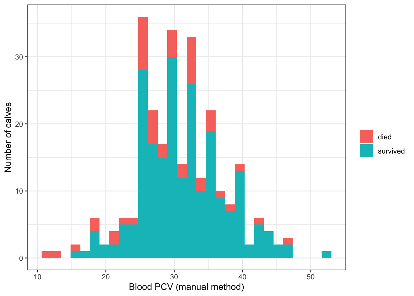 ### Boxplots
- Boxplots are often used in explanatory data analysis and aid in showing the shape of the distribution of the data, the central value and variability, while highlighting the outliers.
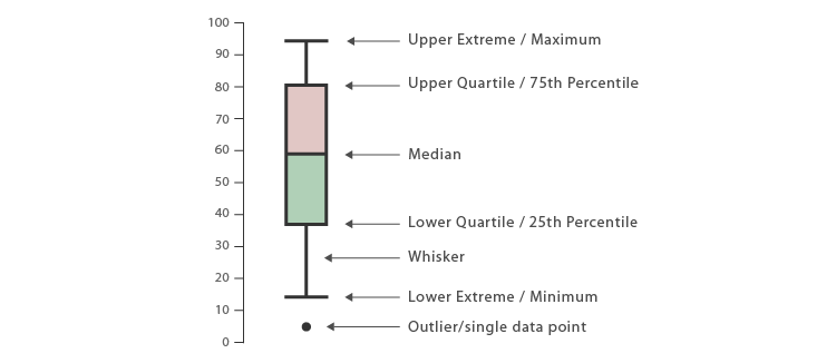
Source: visualoop.com
- The image above explains the anatomy of a boxplot. Observations that are 1.5 times more or less than the interquartile range are termed as outliers.
5.1.3.2 geom_boxplots
- We use the geom_boxplot() function to visualise boxplots in ggplot2.
ggplot(ideal, aes(ReasonsLoss1, ManualPCV)) + theme_bw() +
  geom_boxplot()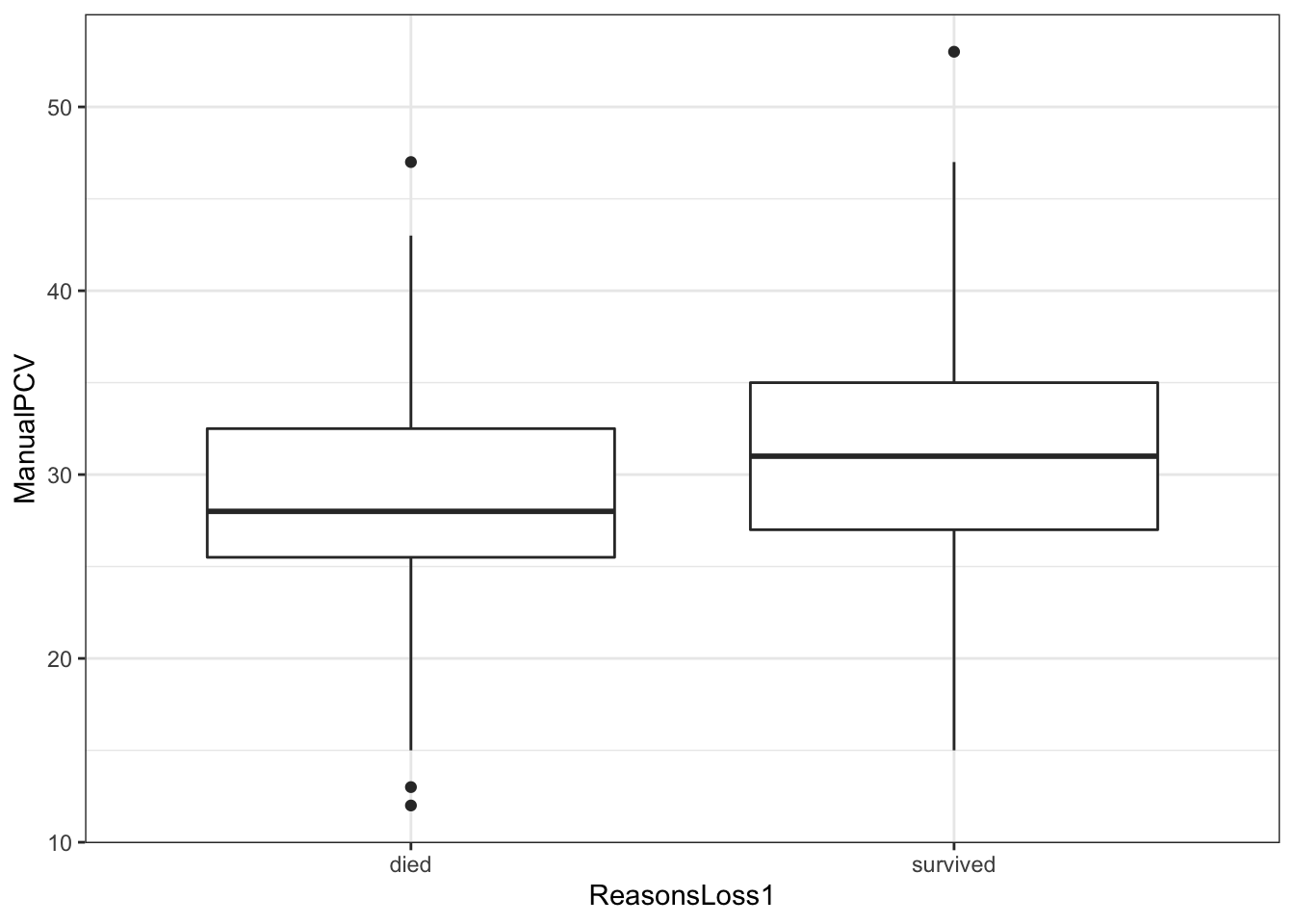
- From our graphic, we can see that we have outliers while the calves that survived had a higher median of the pack cell volume compared to calves that died.
5.1.4 Density plots
These plots are used to observe the distribution of a variable. To visualise them, you require to input one variable, the x axis.
In our case, we will use the density plots to visualise the pack cell volume of the calves per sex.
We will also create an object called niceplot1 that containes the graphic.
ideal<- ideal%>%
  mutate(CalfSex1=recode(CalfSex, "1"="Male", "2"="Female"))

niceplot1 <- ggplot(ideal, aes(x=ManualPCV, fill=CalfSex1)) + theme_bw() +
  #geom_histogram() +
  facet_wrap(Education~ReasonsLoss1) +
  geom_density(alpha = 0.5) +
  labs(y = "Number of calves", x = "ManualPCV")
niceplot1 # object containing the graphic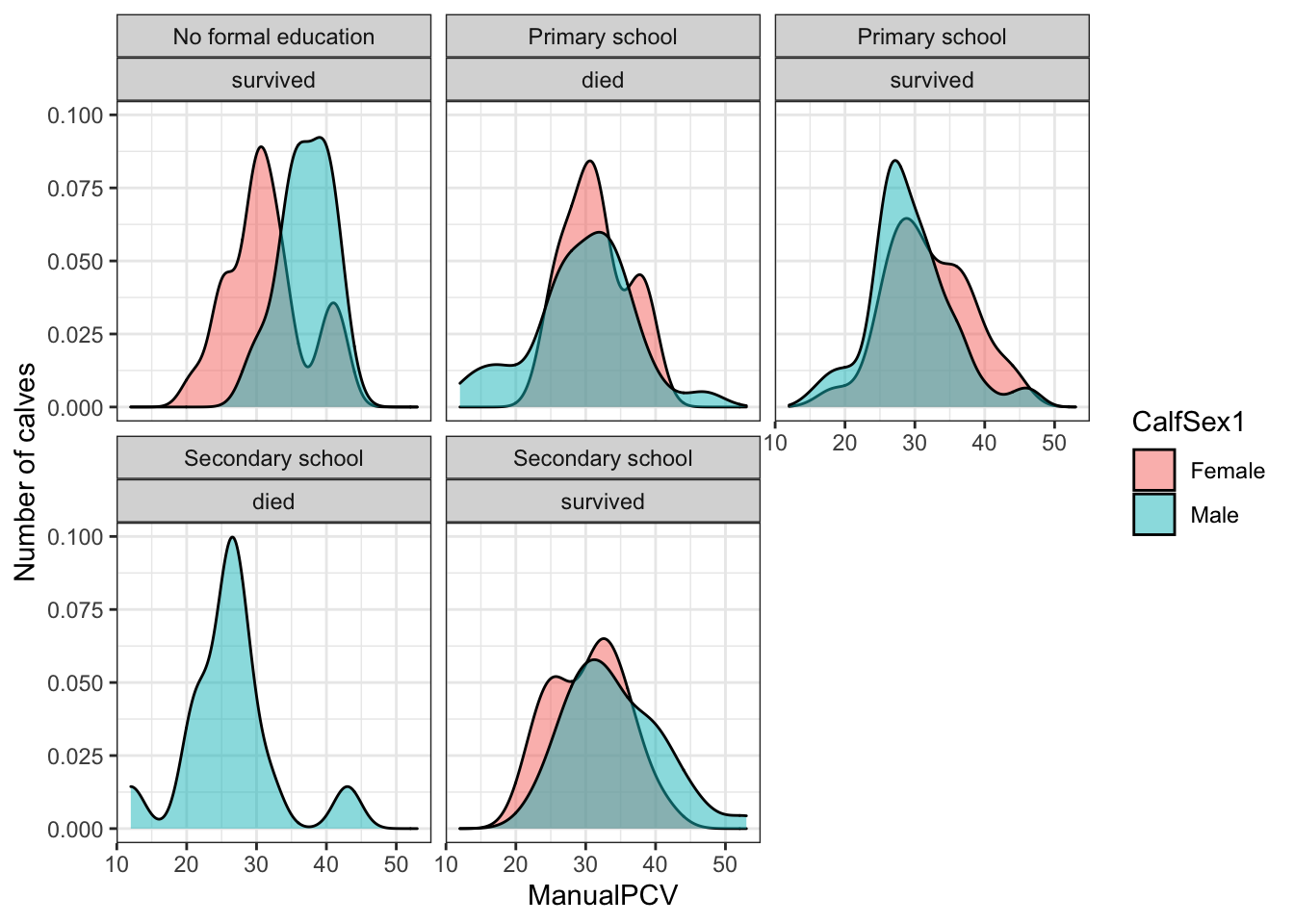
ggplot2 enables one to save graphics from R environmtn to your computer. It gives the user the freedom to choose the format they want to save the graphic in, the resolution and the size.
The beautiful function that enables us to do this is called ggsave() and these graphics are saved in your working environment.
By default, R saves the graphics in a resolution of 300 (which is required by many journals) and when one does not specify the width and height, it gives a default based on the graphic. The graphics saved from R are usually of good quality and may be ued in publications.
Uncomment the line below and try it in your computer. Remember to first set the working directory.
#ggsave("density_graphics.png",niceplot1, dpi=600) # change the dpi to 300 and see how the graphic is.5.1.5 Scatter plots
These plots are used when one has two or more variables that pair well together.
To visualise scatter plots, we will sue the inbuilt dataset iris. You can type this on your console to learn more about this dataset ?iris
5.1.5.1 geom_point
data(iris) # import the data to your global environment

ggplot(iris, aes(x = Petal.Length, y = Sepal.Width)) +
  geom_point()+theme_bw() # cusomtize your x and y axis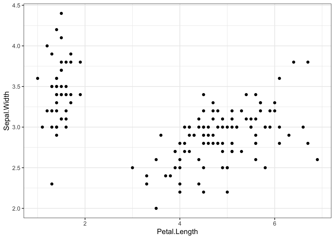
-We can also add color to our scatter plot
ggplot(iris, aes(x = Petal.Length, y = Sepal.Width, colour = Species)) +
  geom_point()+theme_bw()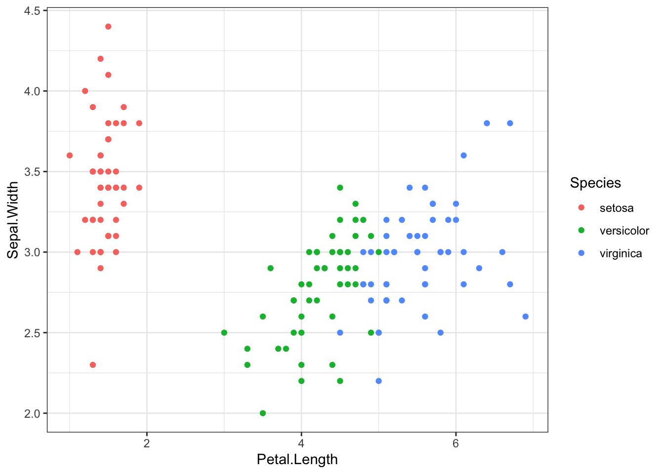
- Or even change the size of the points
ggplot(iris, aes(x = Petal.Length, y = Sepal.Width, col = Species, size = Petal.Width)) +
  geom_point()+theme_bw()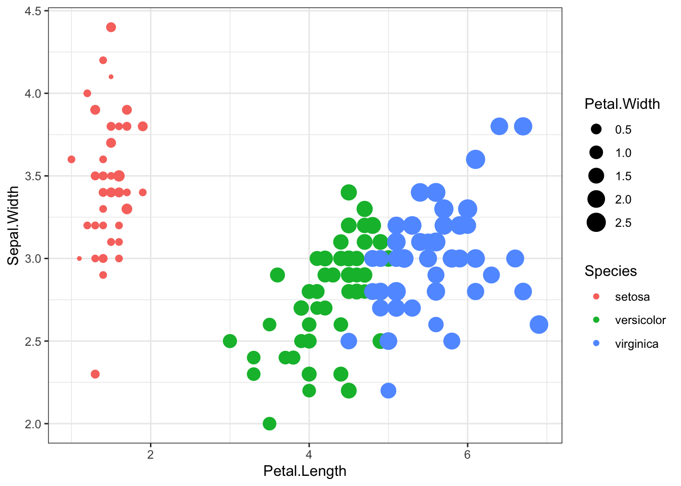
- And the shape of the points
ggplot(iris, aes(x = Petal.Length, y = Sepal.Width, col = Species,
                 size = Petal.Width, shape = Species)) +
  geom_point()+theme_bw()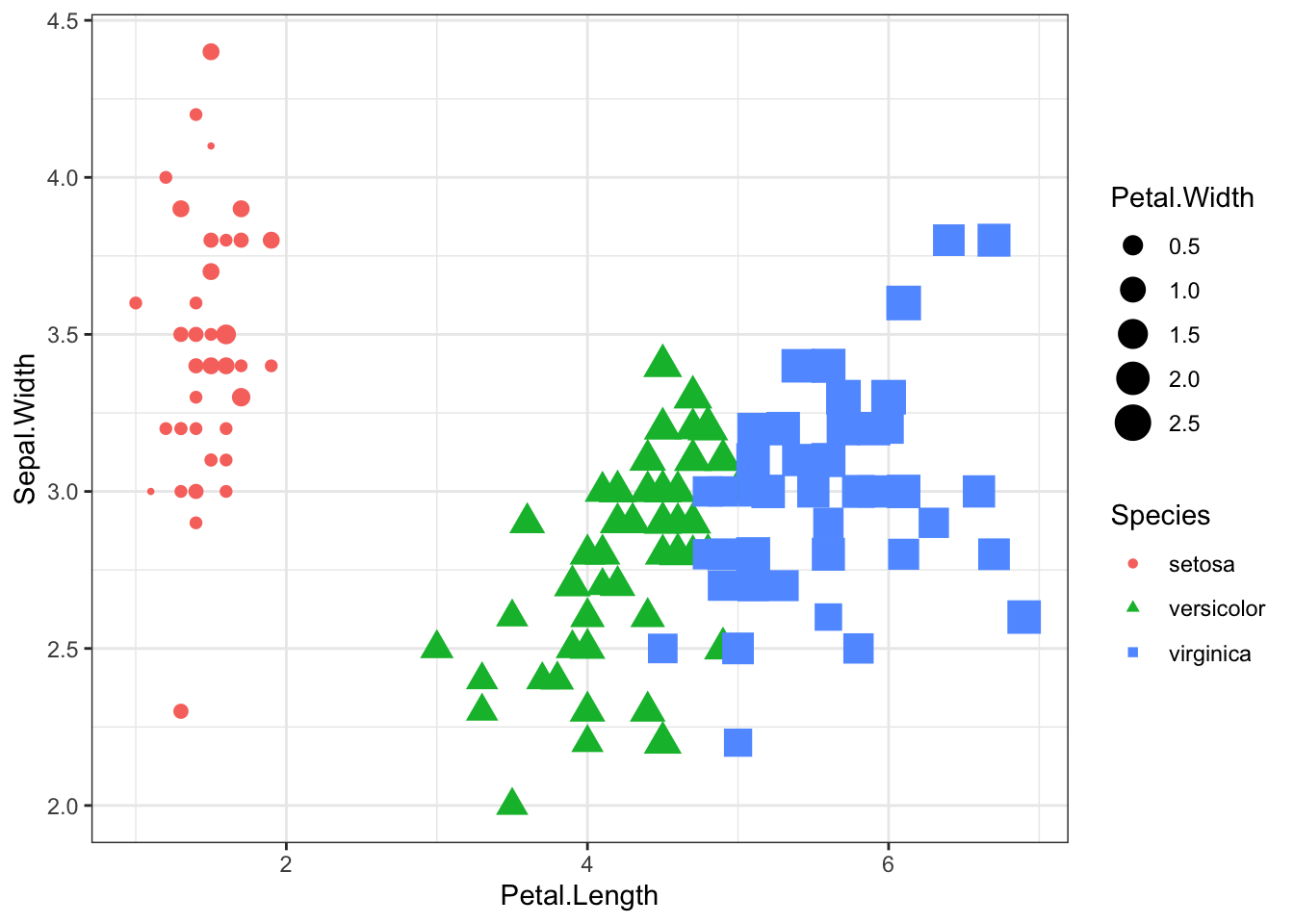
- Or the color intensity
ggplot(iris, aes(x = Petal.Length, y = Sepal.Width, col = Species,
                 size = Petal.Width, shape = Species, alpha = Sepal.Length)) +
  geom_point()+theme_bw()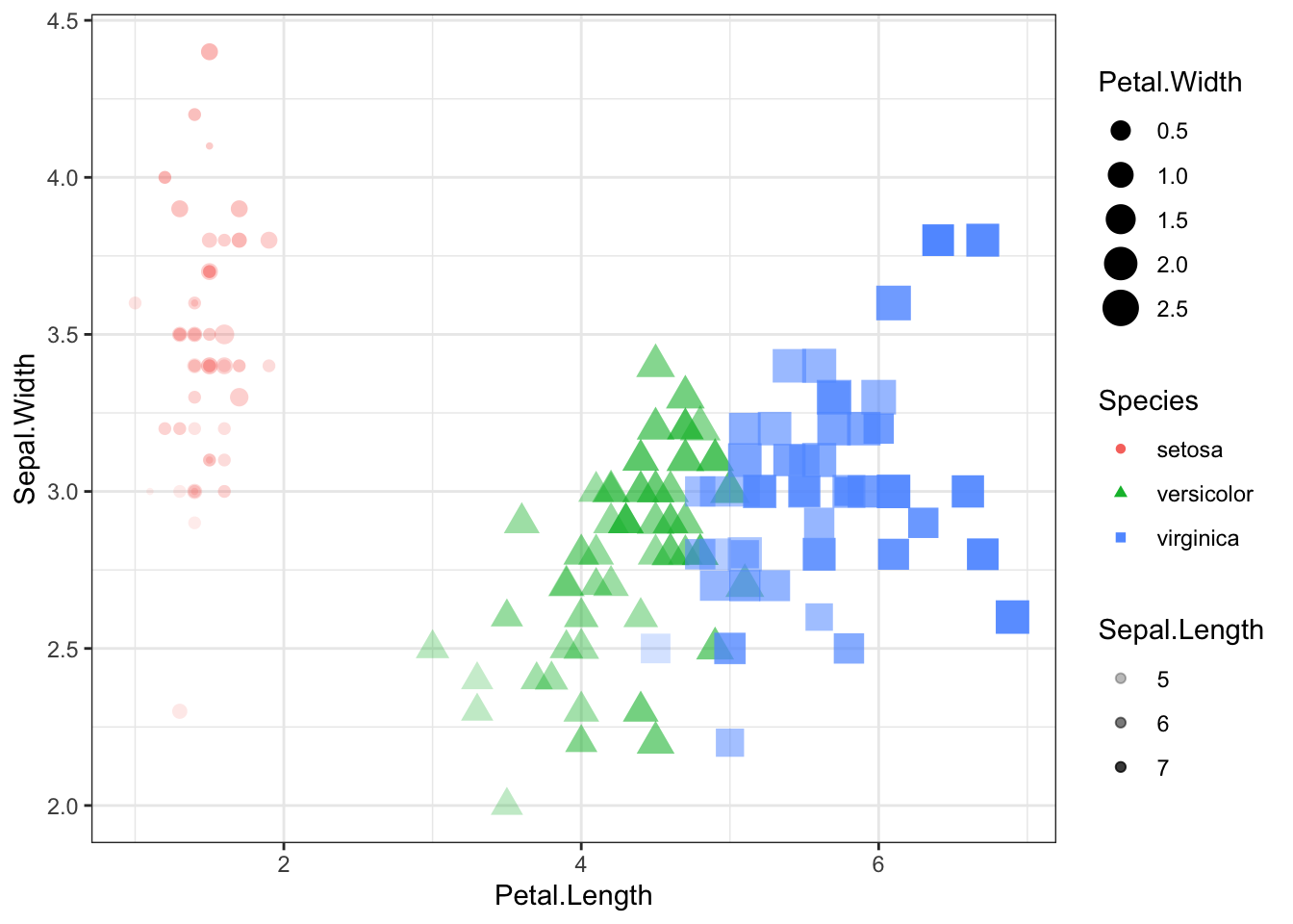
- You can even add statics on your graphics, as seen in the graphs below
ggplot(iris, aes(Species, Sepal.Length)) +
  geom_bar(stat = "summary", fun.y = "mean", fill="blue")+theme_bw()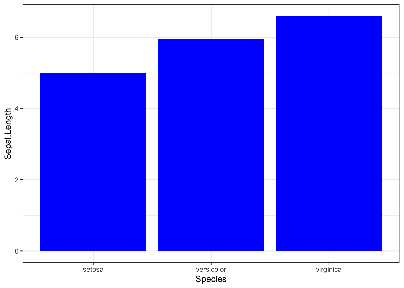
- And even combine more than one visualisation
ggplot(iris, aes(Species, Sepal.Length)) +
  geom_bar(stat = "summary", fun.y = "mean", fill = "#ff0080", col = "black") +
  geom_point()+theme_bw()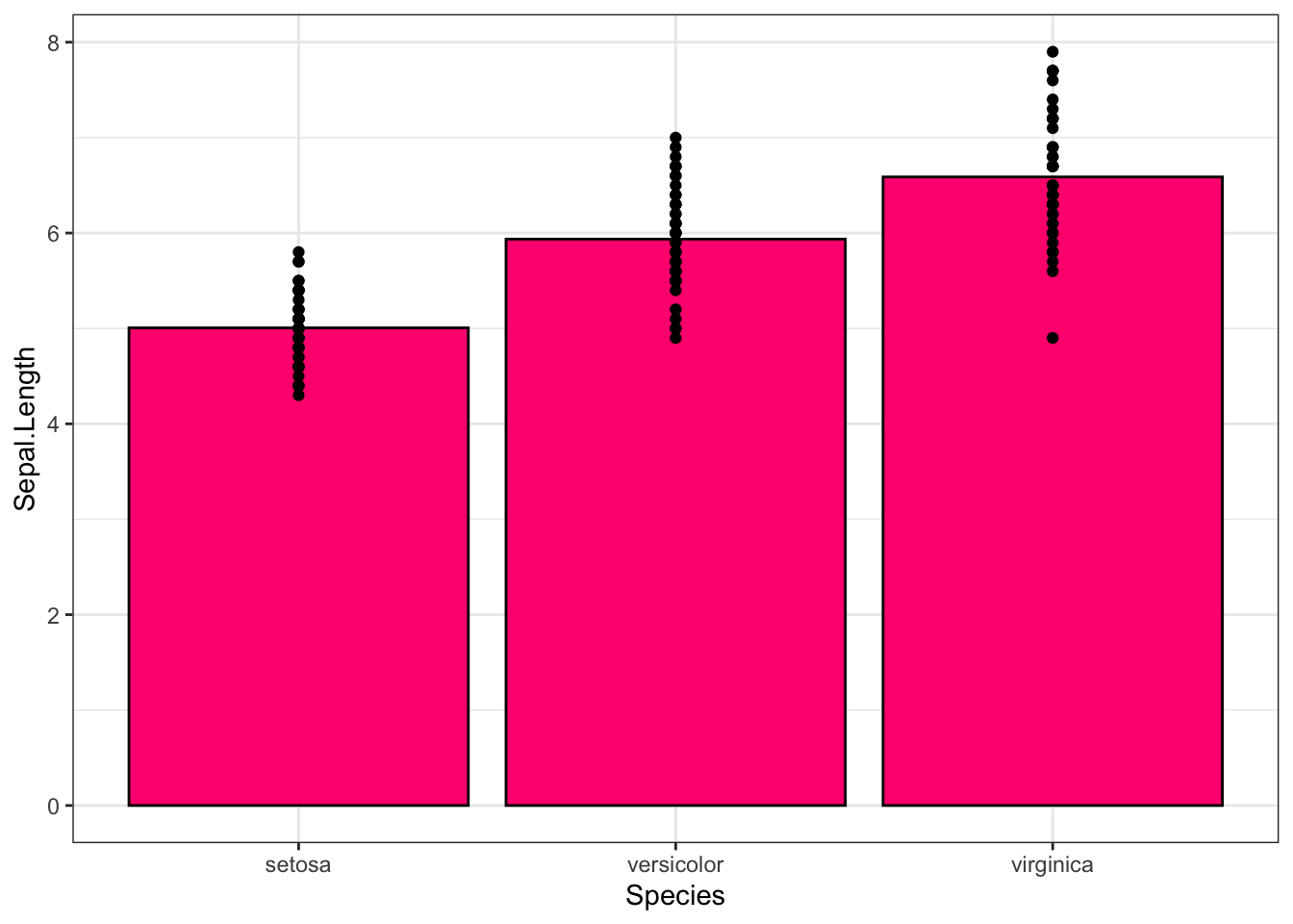
ggplot(iris, aes(Species, Sepal.Length)) +
  geom_bar(stat = "summary", fun.y = "mean", fill = "gray40", col = "black") +
  #geom_point() +
  geom_point(position = position_jitter(0.2), size = 3, shape = 21)+theme_bw()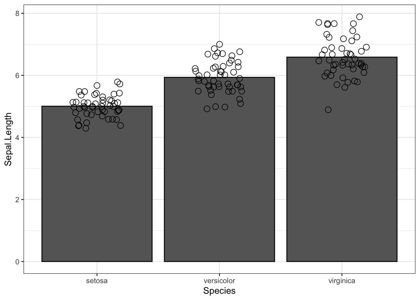
5.1.5.2 More graphic customization
ggplot2 package gives the user the power to customise the graphics to their own liking. This is especially where one would like to change the position of the legend, the size of the text, bolding the text etc.
The theme() function has alot of capability and I would urge you to go to your console and type ?theme to see how much power you have in your hands.
We can try to first change the color of the background of out graphics and the size of the panel border.
niceplot <- ggplot(iris, aes(Species, Sepal.Length)) +
  geom_bar(stat = "summary", fun.y = "mean", fill = "blue", col = "black") +
  geom_point(position = position_jitter(0.2), size = 3, shape = 21)+theme_bw()

niceplot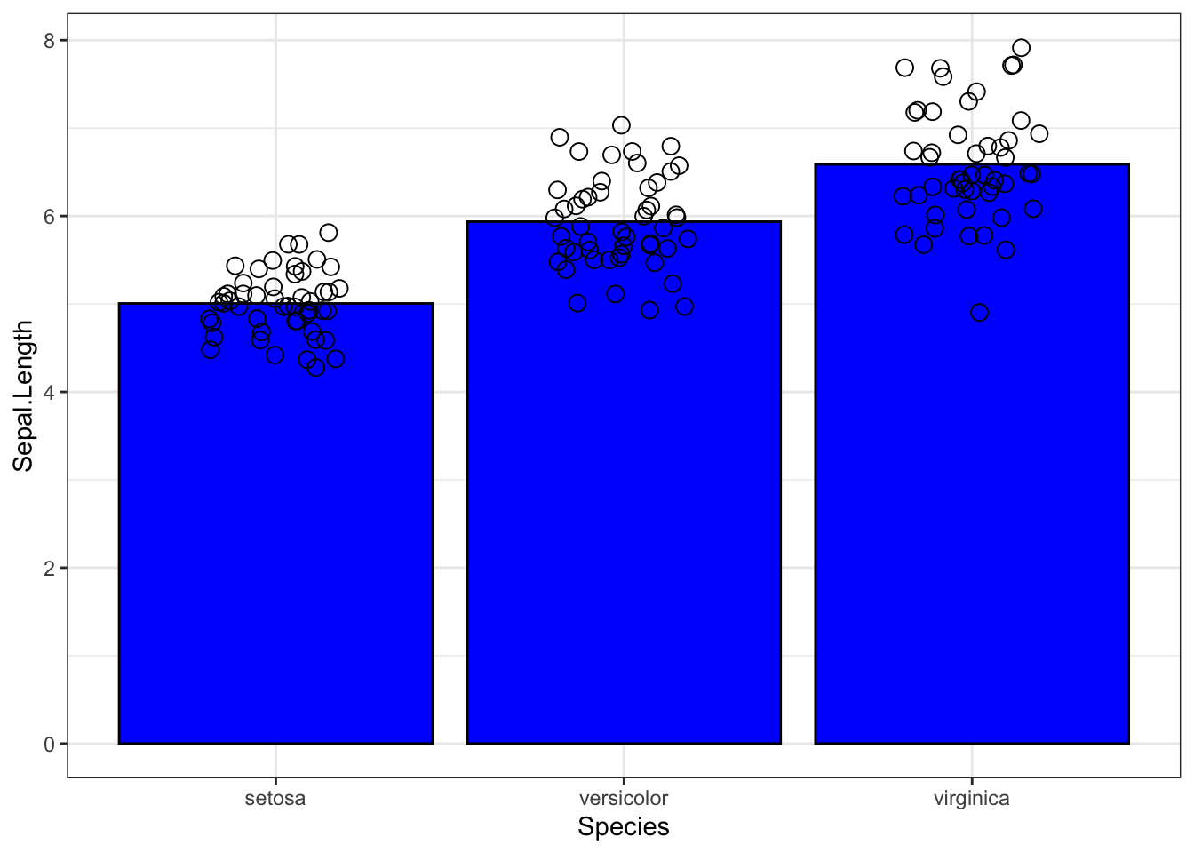
niceplot + theme(panel.grid = element_blank(),
               panel.background = element_rect(fill = "red"),
               panel.border = element_rect(colour = "blue", fill = NA, size = 0.2))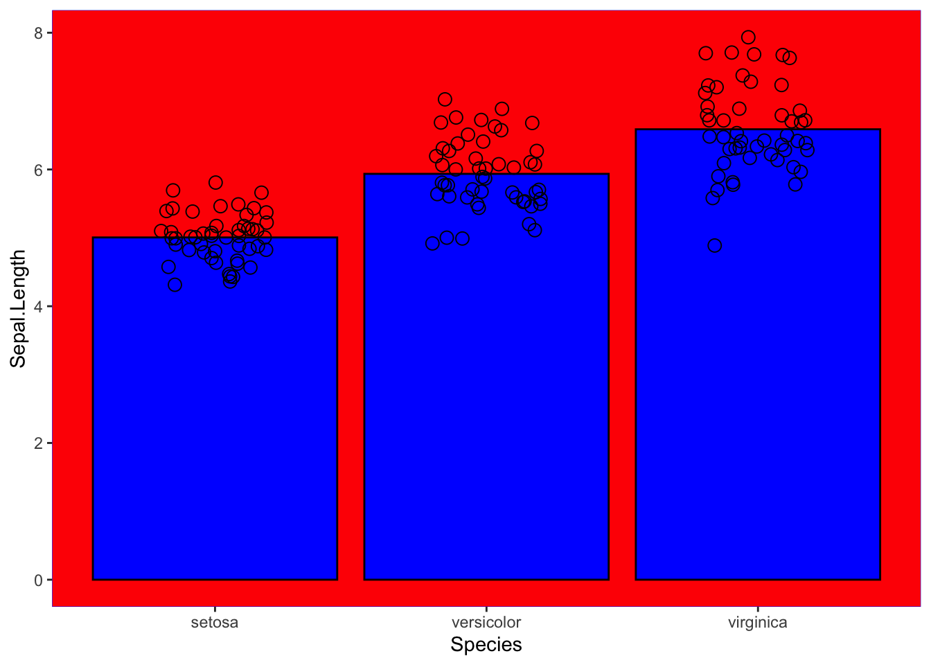
- We can also try and increase the font size of the text and bold them.
ggplot(ideal_data1, aes(x = VisitDate1, y=ADWG1, color=CalfSex)) +
  geom_smooth()+theme_bw()+ scale_x_date(date_breaks = "6 months", date_labels = "%b-%Y")+
  labs(x= "Period (Month-Year)", y="Average daily weight gain", color="Calf Sex")+
  theme(text=element_text(size=14, face="bold"))+ # increase the font and bold the text
  theme(legend.position = "bottom")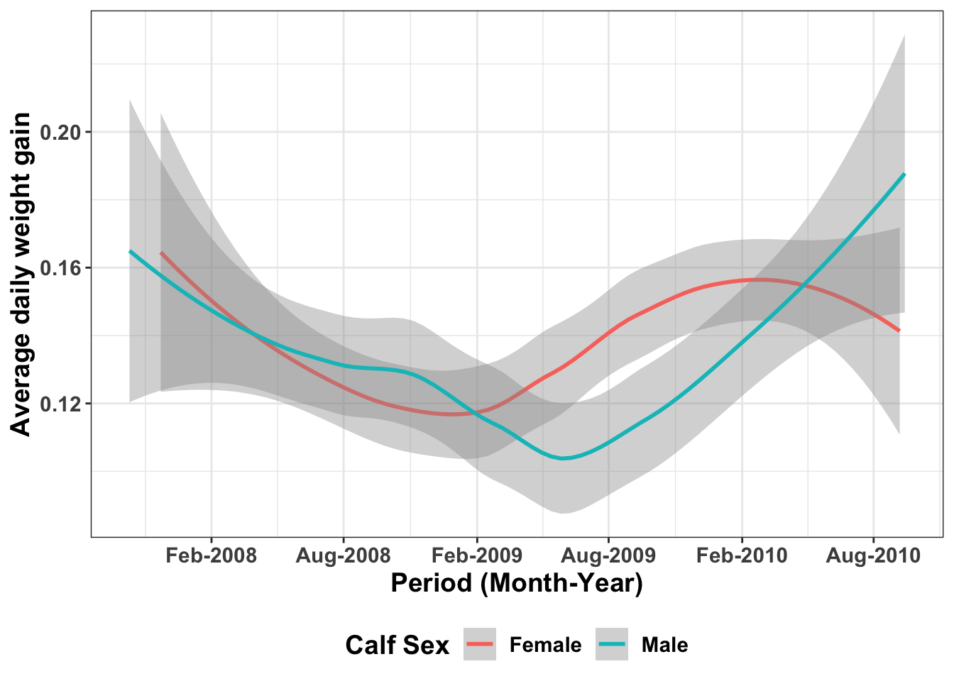
5.1.5.3 Color customisation in graphics
If you look at the graphics above, we have been using the primary colors, as R understands them. However, you may be bold and want to explore more color options. R understands colors in hexagon format and you can use this website called !https://colorbrewer2.org/#type=sequential&scheme=BuGn&n=3 that helps you get the hexagon value of a color while enabling you choose color schemes that are colorblind safe, printer friendly or photocopy safe. These colors are also supported in R and we will try to use them in the visualisation below.
We will use the graph above and change the colors. To see the different color palettes, type this in your console ?scale_color_brewer() or ?scale_fill_brewer()
ggplot(ideal_data1, aes(x = VisitDate1, y=ADWG1, color=CalfSex)) +
geom_smooth()+theme_bw()+ scale_x_date(date_breaks = "6 months", date_labels = "%b-%Y")+
labs(x= "Period (Month-Year)", y="Average daily weight gain", color="Calf Sex")+
theme(text=element_text(size=14, face="bold"))+
theme(legend.position = "bottom")+
scale_color_brewer(palette="RdYlBu")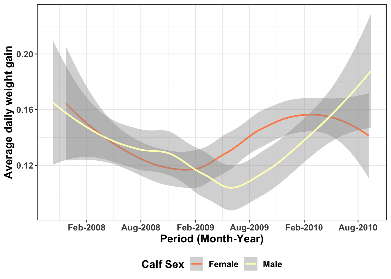 - If you want to add your own colors, yoi can do that manually using the function scale_color_manual() or scale_fill_manual()
ggplot(ideal_data1, aes(x = VisitDate1, y=ADWG1, color=CalfSex)) +
  geom_smooth()+theme_bw()+ scale_x_date(date_breaks = "6 months", date_labels = "%b-%Y")+
  labs(x= "Period (Month-Year)", y="Average daily weight gain", color="Calf Sex")+
  theme(text=element_text(size=14, face="bold"))+
  theme(legend.position = "bottom")+
  scale_color_manual(values=c("#d8b365", "#5ab4ac"))