---
title: "Ministry of Health Department of Family Health"
output:
flexdashboard::flex_dashboard:
orientation: rows
social: menu
source_code: embed
vertical_layout: scroll
self_contained: false
# logo: cema_gok.jpg
---
```{r setup, include=FALSE}
#load packages
library(flexdashboard)
library(tidyverse)
library(shiny)
library(sf)
library(reshape2)
library(cowplot)
library(readxl)
library(treemapify)
library(lubridate)
library(ggiraph)
knitr::opts_chunk$set(echo = FALSE)
knitr::opts_chunk$set(warning = FALSE)
knitr::opts_chunk$set(tidy = TRUE)
knitr::opts_chunk$set(message=FALSE, dev = "png")
county<- st_read("County.shp")
```
Kenya adolescent household survey {data-navmenu="Adolescent and School Health"}
============================================================
Inputs {.sidebar}
-----------------------------------
[Summary](#summary)
[Household characteristics](#household_characteristics)
[Social Demographic characteristics](#sd_characteristics)
[Social characteristics](#social_characteristics)
[Adolescent Nutrition](#adolescent_nutrition)
[Physical Activity](#physical_activity)
[Adolescents Mental Health Status](#mental_status)
[General Adolescent Morbidity](#morbidity)
[Oral Health](#oral_health)
[Injuries](#injuries)
[Child Functioning/Disability](#child_functioning)
[Adolescent Sexual & Reproductive Health](#sexual_health)
[Adolescent HIV](#hiv)
[Adolescent Mortality](#mortality)
```{r, echo=FALSE, out.width='80%'}
knitr::include_graphics("gok_logo.png")
```
```{r, echo=FALSE, out.width='85%'}
knitr::include_graphics("cema_logo.png")
```
summary {.hidden}
==================
Inputs {.sidebar}
-----------------------------------
[Summary](#summary)
[Household characteristics](#household_characteristics)
[Social Demographic characteristics](#sd_characteristics)
[Social characteristics](#social_characteristics)
[Adolescent Nutrition](#adolescent_nutrition)
[Physical Activity](#physical_activity)
[Adolescents Mental Health Status](#mental_status)
[General Adolescent Morbidity](#morbidity)
[Oral Health](#oral_health)
[Injuries](#injuries)
[Child Functioning/Disability](#child_functioning)
[Adolescent Sexual & Reproductive Health](#sexual_health)
[Adolescent HIV](#hiv)
[Adolescent Mortality](#mortality)
```{r, echo=FALSE, out.width='80%'}
knitr::include_graphics("gok_logo.png")
```
```{r, echo=FALSE, out.width='85%'}
knitr::include_graphics("cema_logo.png")
```
Row
---------------------
### Summary
A cross sectional survey was conducted by the Division of Asolescent and School Health (DASH) to assess the health-related knowledge, attitude, behaviour, demographic and clinical characteristics, as well as access to services, among the adolescents aged 10 to 19 years in Kenya. The survey was conducted in 2,953 households where 3,369 adolescents were interviewed in the 44 counties and grouped into 11 regions as seen in the map.
The survey had four objectives:
* To determine the health status of adolescents in Kenya
* To determine the quality of adolescent health services at the health facilities, schools and the community
* To determine the coverage of adolescent health services
* To determine the barriers and enablers to adolescents accessing adolescent health services
As at 2019, there were 47,564,296 people in Kenya,of which 11,631,929 (24%) are adolescents (aged 10-19 years).
Row
---------------------
### Regions in the study
```{r, include=FALSE}
region <- st_read("ke_region.shp")
county <- st_read('County.shp')
pop <- read_csv("survey_pop.csv")
county <- county %>%
left_join(pop, by=c("Name"="county")) %>%
mutate(region=ifelse(Name%in%c("Kiambu", "Kirinyaga","Muranga","Nyandarua", "Nyeri"),
"Central", ifelse(Name%in%c("Kilifi","Kwale","Lamu", "Mombasa","Taita Taveta", "Tana River" ), "Coastal",
ifelse(Name%in%c("Samburu", "Turkana","West Pokot"),"Rift Valley North",
ifelse(Name%in%c("Kisumu", "Siaya"),"Nyanza Central",
ifelse(Name%in%c("Kitui","Machakos","Makueni"),"Lower Eastern",
ifelse(Name%in%c("Garissa", "Mandera","Marsabit", "Wajir"),"North Eastern",
ifelse(Name%in%c("Homa Bay","Kisii", "Migori","Nyamira"), "Nyanza South",
ifelse(Name%in%c("Bungoma", "Busia","Kakamega","Vihiga"), "Western",
ifelse(Name%in%c("Baringo","Bomet","Elgeyo Marakwet","Kajiado","Kericho","Laikipia",
"Nakuru","Nandi", "Narok", "Trans Nzoia", "Uasin Gishu"),"Rift Valley South",
ifelse(Name%in%"Nairobi", "Nairobi","Upper Eastern")))))) ))))) %>%
mutate(pop1=paste0(Name,"\n", pop))
```
```{r, fig.height=8, fig.width=6}
plot <-ggplot(county, aes(label=Name, label1=pop))+geom_sf(aes(fill=region))+theme_void()+
scale_fill_brewer(palette = "Set3")+labs(fill="Region")+theme(text=element_text(size=13))
plotly::ggplotly(plot)
```
Row
----------------------------------
### About the Division of Adoleschent and School Health
The Division of Adolescent and School Health (DASH) is a division of Kenya Ministry of Health under the Directorate of Family Health in the State Department of Medical Services.
**Vision**
A Kenya where all school age children and adolescents are healthy, productive, and live to their fullest potential for national development.
**Mission**
To provide leadership and participate in the implementation of quality evidence-based high impact promotive, preventive, curative and rehabilitative health interventions to all school age children and adolescents
**Mandate**
- Review and development of policies, strategies, and guidelines
- Program planning and budgeting
- Implementation of programs/projects
- Capacity building and technical assistance
- Developing and maintaining quality and standards
- Advocacy, communication, and social mobilization
- Promoting Child and - Adolescent Health rights and responsibilities
- Partnerships and Co-ordination
- Resource mobilization
- Research
- Monitoring and evaluation
**Platforms**
The Division of Adolescent and School Health uses the following platforms to ensure service delivery to adolescents and school age children:
- Inpatient, outpatient, adolescent and youth friendly clinics in public and private healthcare facilities
- Primary and Secondary Schools and other learning institutions like Early Childhood Development Centers and Universities
- Community Health Units
- E-health and M-health services
household_characteristics {.hidden}
==================
Inputs {.sidebar}
-----------------------------------
[Summary](#summary)
[Household characteristics](#household_characteristics)
[Social Demographic characteristics](#sd_characteristics)
[Social characteristics](#social_characteristics)
[Adolescent Nutrition](#adolescent_nutrition)
[Physical Activity](#physical_activity)
[Adolescents Mental Health Status](#mental_status)
[General Adolescent Morbidity](#morbidity)
[Oral Health](#oral_health)
[Injuries](#injuries)
[Child Functioning/Disability](#child_functioning)
[Adolescent Sexual & Reproductive Health](#sexual_health)
[Adolescent HIV](#hiv)
[Adolescent Mortality](#mortality)
```{r, echo=FALSE, out.width='80%'}
knitr::include_graphics("gok_logo.png")
```
```{r, echo=FALSE, out.width='85%'}
knitr::include_graphics("cema_logo.png")
```
Row {.tabset}
------------------------------------------------------------------------------
### Dwelling Characterstics: Floor
```{r dwelling1, fig.width=14, fig.height=8}
dwelling_data <- read_csv("dwelling_data.csv")
dwelling_data1 <- dwelling_data%>%
select(`House Characteristics`,Type,Rural,Urban)%>%
pivot_longer(cols=c("Rural","Urban"), names_to="Residency",values_to = "Proportion")
ggplot(dwelling_data1%>%filter(`House Characteristics`%in%"Floor"),aes(x=reorder(Type, Proportion), y=Proportion, fill=Residency))+
geom_col(position="dodge")+
#facet_wrap(.~`House Characteristics`)+
theme_bw()+
labs(x="Type", y="Proportion (%)", title="",fill="Residency")+
scale_fill_brewer(palette = "Set1")+
theme(text=element_text(size=15))+
coord_flip()
```
### Roofing
```{r dwelling2, fig.width=14, fig.height=8}
ggplot(dwelling_data1%>%filter(`House Characteristics`%in%"Roofing"),aes(x=reorder(Type,Proportion), y=Proportion,fill=Residency))+
geom_col(position="dodge")+
#facet_wrap(.~`House Characteristics`)+
theme_bw()+
labs(x="Type", y="Proportion (%)", title="",fill="Residency")+
scale_fill_brewer(palette = "Set1")+
theme(text=element_text(size=15))+
coord_flip()
```
### Sleeping Rooms
```{r dwelling3, fig.width=14, fig.height=8}
dwelling_data1$Type <- fct_relevel(dwelling_data1$Type, "Zero", "One", "Two", "Three or more")
ggplot(dwelling_data1%>%filter(`House Characteristics`%in%"Sleeping Rooms"),aes(x=Type, y=`Proportion`,fill=Residency))+
geom_col(position="dodge")+
#facet_wrap(.~`House Characteristics`)+
theme_bw()+
labs( y="Proportion (%)", title="",fill="Residency")+
scale_fill_brewer(palette = "Set1")+
theme(text=element_text(size=15))+
coord_flip()
```
### Wall
```{r dwelling4, fig.width=14, fig.height=8}
ggplot(dwelling_data1%>%filter(`House Characteristics`%in%"Wall"),aes(x=reorder(Type,Proportion), y=Proportion))+
geom_col(position="dodge", fill="#377eb8")+
facet_wrap(.~Residency)+
theme_bw()+
labs( y="Proportion (%)", x="Type",title="",fill="Residency")+
scale_fill_brewer(palette = "Set1")+
theme(text=element_text(size=15))+
coord_flip()
```
Row {.tabset}
------------------------------------------------------------------------------
### Water Source Type
```{r wash1, fig.width=14}
wash_data <- read_csv("wash_data.csv")
wash_data1 <- wash_data%>%
select(`House Characteristics`,Type,Rural,Urban)%>%
pivot_longer(cols=c("Rural","Urban"), names_to="Residency",values_to = "Proportion")
ggplot(wash_data1%>%filter(`House Characteristics`%in%"Water source type"),aes(x=Type, y=`Proportion`,fill=Residency))+
geom_col(position="dodge")+
#facet_wrap(.~`House Characteristics`)+
theme_bw()+
labs( y="Proportion (%)", title="",fill="Residency")+
scale_fill_brewer(palette = "Set1")+
theme(text=element_text(size=15))+
coord_flip()
```
### Water Treatment Methods
```{r wash2, fig.width=14}
ggplot(wash_data1%>%filter(`House Characteristics`%in%"Water treatment methods"),aes(x=Type, y=`Proportion`,fill=Residency))+
geom_col(position="dodge")+
#facet_wrap(.~`House Characteristics`)+
theme_bw()+
labs( y="Proportion (%)", title="",fill="Residency")+
scale_fill_brewer(palette = "Set1")+
theme(text=element_text(size=15))+
coord_flip()
```
### Toilet type
```{r wash3, fig.width=14}
ggplot(wash_data1%>%filter(`House Characteristics`%in%"Toilet type"),aes(x=reorder(Type,Proportion), y=`Proportion`,fill=Residency))+
geom_col(position="dodge")+
#facet_wrap(.~`House Characteristics`)+
theme_bw()+
labs(x="Type", y="Proportion (%)", title="",fill="Residency")+
scale_fill_brewer(palette = "Set1")+
theme(text=element_text(size=15))+
coord_flip()
```
Row {.tabset}
------------------------------------------------------------------------------
### WASH indicators
```{r wash4, fig.width=14}
wash_data2 <- wash_data%>%
select(`House Characteristics`,Type,Central:National)%>%
pivot_longer(cols=c("Central":"National"), names_to="Region",values_to = "Proportion") %>%
filter(Region!="National")
wash_county<- full_join(region, wash_data2%>%filter(`House Characteristics`%in%c("Treat (make it safe) water prior drinking","Latrine shared with other")), by=c("region"="Region"))
ggplot(wash_data2%>%filter(`House Characteristics`%in%c("Treat (make it safe) water prior drinking","Latrine shared with other")),aes(x=Region, y=`Proportion`,fill=Type))+
geom_col()+
facet_wrap(.~`House Characteristics`)+
theme_bw()+
labs( y="Proportion (%)", title="",fill="")+
scale_fill_brewer(palette = "Set1")+
theme(text=element_text(size=15))+
coord_flip()
```
### WASH indicators- map
```{r, fig.width=18}
ggplot(wash_county[wash_county$Type%in%"Yes",], aes(fill=Proportion))+geom_sf()+facet_grid(.~`House Characteristics`)+theme_void()+scale_fill_gradient(low="#d73027", high="#4575b4", na.value = "white")+geom_sf_text(aes(label=round(Proportion)), check_overlap = T)
```
### Location of water source
```{r wash5, fig.width=14}
location_county<- full_join(region, wash_data2%>%filter(`House Characteristics`%in%"Location of water source"), by=c("region"="Region"))
ggplot(wash_data2%>%filter(`House Characteristics`%in%"Location of water source"),aes(x=Region, y=`Proportion`,fill=Type))+
geom_col()+
#facet_wrap(.~`House Characteristics`)+
theme_bw()+
labs( y="Proportion (%)", title="",fill="")+
scale_fill_brewer(palette = "Set1")+
theme(text=element_text(size=15))+
coord_flip()
```
### Location of water source - Map
```{r, fig.width=16}
ggplot(location_county, aes(fill=Proportion))+geom_sf()+theme_void()+
facet_grid(.~Type)+theme_void()+scale_fill_gradient(low="#d73027", high="#4575b4", na.value = "white")+geom_sf_text(aes(label=round(Proportion)), check_overlap = T)
```
### Number of households sharing latrine
```{r wash6, fig.width=14}
latrine_county<- full_join(region, wash_data2%>%filter(`House Characteristics`%in%"Number of households sharing latrine"), by=c("region"="Region"))
ggplot(wash_data2%>%filter(`House Characteristics`%in%"Number of households sharing latrine"),aes(x=Region, y=`Proportion`,fill=Type))+
geom_col()+
#facet_wrap(.~`House Characteristics`)+
theme_bw()+
labs( y="Proportion (%)", title="",fill="")+
scale_fill_brewer(palette = "Set1")+
theme(text=element_text(size=15))+
coord_flip()
```
### Number of households sharing latrine - Map
```{r, fig.width=16}
ggplot(latrine_county, aes(fill=Proportion))+geom_sf()+theme_void()+
facet_grid(.~Type)+theme_void()+scale_fill_gradient(low="#d73027", high="#4575b4", na.value = "white")+geom_sf_text(aes(label=round(Proportion)), check_overlap = T)
```
Row {.tabset}
------------------------------------------------------------------------------
### Source of cooking fuel
```{r cooking1, fig.width=14}
cooking_data <- read_csv("cooking_data.csv")
cooking_data1 <- cooking_data%>%
select(`Characteristics`,Type,Rural,Urban)%>%
pivot_longer(cols=c("Rural","Urban"), names_to="Residency",values_to = "Proportion")
ggplot(cooking_data1%>%filter(`Characteristics`%in%"Source of cooking fuel"),aes(x=reorder(Type, Proportion), y=`Proportion`,fill=Residency))+
geom_col(position="dodge")+
#facet_wrap(.~`House Characteristics`)+
theme_bw()+
labs(x="Type", y="Proportion (%)", title="",fill="Residency",x="")+
scale_fill_brewer(palette = "Set1")+
theme(text=element_text(size=15))+
coord_flip()
```
### Place of cooking
```{r cooking2, fig.width=14}
cooking_data2 <- cooking_data%>%
select(`Characteristics`,Type,Central:National)%>%
pivot_longer(cols=c("Central":"National"), names_to="Region",values_to = "Proportion") %>%
filter(Region!="National")
cooking_county<- full_join(region, cooking_data2%>%filter(`Characteristics`%in%"Place of cooking"), by=c("region"="Region"))
ggplot(cooking_data2%>%filter(`Characteristics`%in%"Place of cooking"),aes(x=reorder(Region, Proportion), y=`Proportion`,fill=Type))+
geom_col()+
#facet_wrap(.~`Characteristics`)+
theme_bw()+
labs( y="Proportion (%)", title="",fill="Place of cooking")+
scale_fill_brewer(palette = "Set1")+
theme(text=element_text(size=15))+
coord_flip()
```
### Place of cooking - Map
```{r, warning=F,fig.width=16}
cooking_county$Type <- fct_relevel(cooking_county$Type, "In a Separate Building", "In the house", "Outdoors", "Other")
ggplot(cooking_county, aes(fill=Proportion))+geom_sf()+theme_void()+
facet_grid(.~Type)+theme_void()+scale_fill_gradient(low="#d73027", high="#4575b4", na.value = "white")+geom_sf_text(aes(label=round(Proportion)), check_overlap = T)
```
Row {.tabset}
------------------------------------------------------------------------------
### Assets ownership by residency
```{r assets1, fig.width=14, fig.height=14}
assets_data <- read_csv("assets_data.csv")
assets_data1 <- assets_data%>%
select(Assets,Rural,Urban)%>%
pivot_longer(cols=c("Rural","Urban"), names_to="Residency",values_to = "Proportion")%>%
mutate(Category="Residency")
ggplot(assets_data1,aes(x=reorder(Assets,Proportion), y=`Proportion`,fill=Residency))+
geom_col(position="dodge")+ylim(0,110)+
#facet_wrap(.~`House Characteristics`)+
theme_bw()+
labs( y="Proportion (%)", title="",fill="Residency",x="")+
scale_fill_brewer(palette = "Set1")+
theme(text=element_text(size=15))+
coord_flip()
```
### Assets ownership by region
```{r assets2, fig.width=14, fig.height=14}
assets_data2 <- assets_data%>%
select(Assets,Central:Western,National)%>%
pivot_longer(cols=c("Central":"Western","National"), names_to="Region",values_to = "Proportion")%>%
mutate(Category="Region") %>%
mutate(Proportion=ifelse(Proportion<0.5, Proportion, round(Proportion)))
assets_data2$Assets <- fct_relevel(assets_data2$Assets, "Mobile phone", "Television","Radio","Bank account ownership", "Watch","Electricity","Solar","Bicycle", "Computer", "Motorcycle/scooter", "Refrigerator", "Car or truck")
ggplot(assets_data2,aes(x=reorder(Region,Proportion), y=round(Proportion),label=`Proportion`))+
geom_col(fill="#4daf4a")+
facet_wrap(.~Assets)+
theme_bw()+
labs( y="Proportion (%)", title="Assets Ownership",fill="",x="Region")+
scale_fill_brewer(palette = "Set1")+
theme(text=element_text(size=15))+
coord_flip()+ylim(0,110)+
geom_text(hjust=-0.2)
```
### Assets ownership by region - Map
```{r, fig.width=14, fig.height=14}
assets_county<- full_join(region, assets_data2, by=c("region"="Region"))
ggplot(assets_county, aes(fill=Proportion))+geom_sf()+theme_void()+
facet_wrap(.~Assets)+theme_void()+scale_fill_gradient(low="#ffffcc", high="#bd0026", na.value = "white")+geom_sf_text(aes(label=round(Proportion)), check_overlap=T)
```
sd_characteristics {.hidden}
==========
Inputs {.sidebar}
-----------------------------------
[Summary](#summary)
[Household characteristics](#household_characteristics)
[Social Demographic characteristics](#sd_characteristics)
[Social characteristics](#social_characteristics)
[Adolescent Nutrition](#adolescent_nutrition)
[Physical Activity](#physical_activity)
[Adolescents Mental Health Status](#mental_status)
[General Adolescent Morbidity](#morbidity)
[Oral Health](#oral_health)
[Injuries](#injuries)
[Child Functioning/Disability](#child_functioning)
[Adolescent Sexual & Reproductive Health](#sexual_health)
[Adolescent HIV](#hiv)
[Adolescent Mortality](#mortality)
```{r, echo=FALSE, out.width='80%'}
knitr::include_graphics("gok_logo.png")
```
```{r, echo=FALSE, out.width='85%'}
knitr::include_graphics("cema_logo.png")
```
Row {.tabset}
------------------------------------------------------------------------------
### Adolescents' Age distribution
```{r demographics1, fig.width=10}
demographic_data <- read_csv("demographic_data.csv")%>%
mutate(Category=recode(Category,"14-Oct"="10-14","5-Jan"="1-5"))
demographic_data1 <- demographic_data%>%
select(Characteristics,Category,Rural,Urban)%>%
pivot_longer(cols=c("Rural","Urban"), names_to="Residency",values_to = "Proportion")%>%
filter(Residency!="National")
demographic_data2 <- demographic_data%>%
select(Characteristics,Category,Central:National)%>%
pivot_longer(cols=c("Central":"National"), names_to="Region",values_to = "Proportion")%>%
filter(Region!="National")
demographic_data3 <- demographic_data%>%
pivot_longer(cols=c("Rural":"National"), names_to="Region",values_to = "Proportion")%>%
filter(Region!="National")
ggplot(demographic_data3%>%filter(`Characteristics`%in%"Age"),aes(x=Region, y=`Proportion`,fill=Category))+
geom_col()+
#facet_wrap(.~`House Characteristics`)+
theme_bw()+
labs( y="Proportion (%)", title="",fill="Age Category")+
scale_fill_brewer(palette = "Set1")+
theme(text=element_text(size=15))+
coord_flip()
```
### Adolescents' Age distribution - Map
```{r, fig.width=16}
age_county<- full_join(region, demographic_data3%>%filter(`Characteristics`%in%"Age"), by=c("region"="Region"))
ggplot(age_county, aes(fill=Proportion))+geom_sf()+theme_void()+
facet_wrap(.~Category)+theme_void()+scale_fill_gradient(low="#ffffcc", high="#bd0026", na.value = "white")+geom_sf_text(aes(label=round(Proportion)), check_overlap=T)
```
### Adolescents' Gender distribution
```{r demographics2, fig.width=10}
ggplot(demographic_data3%>%filter(`Characteristics`%in%"Sex"),aes(x=Region, y=`Proportion`,fill=Category))+
geom_col()+
#facet_wrap(.~`House Characteristics`)+
theme_bw()+
labs( y="Proportion (%)", title="",fill="Gender")+
scale_fill_brewer(palette = "Set1")+
theme(text=element_text(size=15))+
coord_flip()
```
### Adolescents' Gender distribution - Map
```{r, fig.width=16}
sex_county<- full_join(region, demographic_data3%>%filter(`Characteristics`%in%"Sex"), by=c("region"="Region"))
ggplot(sex_county, aes(fill=Proportion))+geom_sf()+theme_void()+
facet_wrap(.~Category)+theme_void()+scale_fill_gradient(low="#ffffcc", high="#bd0026", na.value = "white")+geom_sf_text(aes(label=round(Proportion)),check_overlap=T )+theme(strip.text.x = element_text(size = 15, face="bold"))
```
Row {.tabset}
------------------------------------------------------------------------------
### School Attendance
```{r demographics3, fig.width=10}
ggplot(demographic_data3%>%filter(`Characteristics`%in%c("Ever attended school","Currently enrolled in school")),aes(x=Region, y=`Proportion`,fill=Category))+
geom_col()+
facet_wrap(.~`Characteristics`)+
theme_bw()+
labs( y="Proportion (%)", title="",fill="")+
scale_fill_brewer(palette = "Set1")+
theme(text=element_text(size=15))+
coord_flip()
```
### School Attendance - Map
```{r, fig.width=16}
school_county<- full_join(region, demographic_data3%>%filter(`Characteristics`%in%c("Ever attended school","Currently enrolled in school")), by=c("region"="Region"))
ggplot(school_county[school_county$Category%in%"Yes",], aes(fill=Proportion))+geom_sf()+theme_void()+
facet_wrap(.~Characteristics)+theme_void()+scale_fill_gradient(low="#ffffcc", high="#bd0026", na.value = "white")+geom_sf_text(aes(label=round(Proportion)), check_overlap=T)+theme(strip.text.x = element_text(size = 15, face="bold"))
```
### Highest level of school attended
```{r demographics4, fig.width=10}
demographic_data3$Category <- recode(demographic_data3$Category, "Secondary/'a' level"="Secondary/A level")
demographic_data3$Category <- fct_relevel(demographic_data3$Category, "Primary","Post-primary/vocational", "Secondary/A level", "College (middle level)", "University")
ggplot(demographic_data3%>%filter(`Characteristics`%in%"Highest level of school attended"),aes(x=Region, y=`Proportion`,fill=Category))+
geom_col()+
#facet_wrap(.~`House Characteristics`)+
theme_bw()+
labs( y="Proportion (%)", title="",fill="")+
scale_fill_brewer(palette = "Set1")+
theme(text=element_text(size=15))+
coord_flip()
```
### Highest level of school attended - Map
```{r, fig.width=16}
attendance_county<- full_join(region, demographic_data3%>%filter(`Characteristics`%in%"Highest level of school attended"), by=c("region"="Region"))
attendance_county$Category <- fct_relevel(attendance_county$Category, "Primary","Post-primary/vocational", "Secondary/A level", "College (middle level)", "University")
ggplot(attendance_county, aes(fill=Proportion))+geom_sf()+theme_void()+
facet_grid(.~Category)+theme_void()+scale_fill_gradient(low="#ffffcc", high="#bd0026", na.value = "white")+geom_sf_text(aes(label=round(Proportion)), check_overlap=T)+theme(strip.text.x = element_text(size = 15, face="bold"))
```
### Reading skill (For those with primary school level)
```{r demographics5, fig.width=10}
demographic_data3$Category <- fct_relevel(demographic_data3$Category, "Able to read whole sentence", "Able to read only parts of sentence", "Cannot read at all", "No card with required language")
ggplot(demographic_data3%>%filter(`Characteristics`%in%"Reading skill (For those with primary school level)"),aes(x=Region, y=`Proportion`,fill=Category))+
geom_col()+
#facet_wrap(.~`House Characteristics`)+
theme_bw()+
labs( y="Proportion (%)", title="",fill="")+
scale_fill_brewer(palette = "Set1")+
theme(text=element_text(size=15))+
coord_flip()
```
### Reading skill - Map
```{r, fig.width=16}
reading_county<- full_join(region, demographic_data3%>%filter(`Characteristics`%in%"Reading skill (For those with primary school level)"), by=c("region"="Region"))
attendance_county$Category <- fct_relevel(attendance_county$Category, "Primary","Post-primary/vocational", "Secondary/A level", "College (middle level)", "University")
ggplot(reading_county, aes(fill=Proportion))+geom_sf()+theme_void()+
facet_grid(.~Category)+theme_void()+scale_fill_gradient(low="#ffffcc", high="#bd0026", na.value = "white")+geom_sf_text(aes(label=round(Proportion)),check_overlap=T)+theme(strip.text.x = element_text(size = 15, face="bold"))
```
Row {.tabset}
------------------------------------------------------------------------------
### Number of days missed school in past 3 months
```{r demographics6, fig.width=10}
demographic_data3$Category <- fct_relevel(demographic_data3$Category, "0","1-5",">5")
ggplot(demographic_data3%>%filter(`Characteristics`%in%"Number of days missed school in past 3 months"),aes(x=Region, y=`Proportion`,fill=Category))+
geom_col()+
#facet_wrap(.~`House Characteristics`)+
theme_bw()+
labs( y="Proportion (%)", title="",fill="Number of days")+
scale_fill_brewer(palette = "Set1")+
theme(text=element_text(size=15))+
coord_flip()
```
### Number of days missed school in past 3 months - Map
```{r demographics6a, fig.width=10}
school_county<- full_join(region, demographic_data3%>%filter(`Characteristics`%in%"Number of days missed school in past 3 months"), by=c("region"="Region"))
ggplot(school_county, aes(fill=Proportion))+geom_sf()+theme_void()+
facet_grid(.~Category)+theme_void()+scale_fill_gradient(low="#ffffcc", high="#bd0026", na.value = "white")+geom_sf_text(aes(label=round(Proportion)),check_overlap=T)+theme(strip.text.x = element_text(size = 15, face="bold"))
```
### Reasons for missing school
```{r demographics7, fig.width=10}
ggplot(demographic_data2%>%filter(Region!="National")%>%filter(Characteristics%in%"Reasons for missing school"),aes(x=reorder(Category, Proportion), y=`Proportion`,label=`Proportion`))+
geom_col(fill="#4daf4a")+
facet_wrap(.~Region)+
theme_bw()+
labs( y="Proportion (%)", title="",fill="",x="")+
scale_fill_brewer(palette = "Set1")+
theme(text=element_text(size=15))+
coord_flip()+
geom_text(hjust=-0.3)
```
### Reasons for missing school - Map
```{r demographics7a, fig.width=16}
missing_county<- full_join(region, demographic_data2%>%filter(Region!="National")%>%filter(Characteristics%in%"Reasons for missing school"), by=c("region"="Region"))%>%
filter(Category%in%c("I have been sick","There's not enough money to send me to school"))%>%
mutate(Category=recode(Category, "There's not enough money to send me to school"="There's not enough money \nto send me to school"))
ggplot(missing_county, aes(fill=Proportion))+geom_sf()+theme_void()+
facet_grid(.~Category)+theme_void()+scale_fill_gradient(low="#ffffcc", high="#bd0026", na.value = "white")+geom_sf_text(aes(label=round(Proportion)),check_overlap=T)+theme(strip.text.x = element_text(size = 15, face="bold"))
```
social_characteristics {.hidden}
==========
Inputs {.sidebar}
-----------------------------------
[Summary](#summary)
[Household characteristics](#household_characteristics)
[Social Demographic characteristics](#sd_characteristics)
[Social characteristics](#social_characteristics)
[Adolescent Nutrition](#adolescent_nutrition)
[Physical Activity](#physical_activity)
[Adolescents Mental Health Status](#mental_status)
[General Adolescent Morbidity](#morbidity)
[Oral Health](#oral_health)
[Injuries](#injuries)
[Child Functioning/Disability](#child_functioning)
[Adolescent Sexual & Reproductive Health](#sexual_health)
[Adolescent HIV](#hiv)
[Adolescent Mortality](#mortality)
```{r, echo=FALSE, out.width='80%'}
knitr::include_graphics("gok_logo.png")
```
```{r, echo=FALSE, out.width='85%'}
knitr::include_graphics("cema_logo.png")
```
Row {data-height=200}
------------------------------------------------------------------------------
### ValueBox
```{r}
valueBox(scales::percent(0.77), 'of male adolescents used thier own money on phones and airtime',icon='fa-mobile', color="#D16D2A"
)
```
### ValueBox
```{r}
valueBox(scales::percent(0.715), 'of females invested in business with their own money',icon='fa-briefcase', color="#55A8DC")
```
### ValueBox
```{r}
valueBox(scales::percent(0.021), 'of men spent money on alcohol',icon='fa-beer', color="#D16D2A"
)
```
Row {.tabset}
------------------------------------------------------------------------------
### Male Essential Expenditure
```{r, fig.width=16}
basic_essential_expenditure <- read_csv("essential_expenses.csv")
male_expenditure<-basic_essential_expenditure[c(16:30),c(0:4)]
ggplot(data=male_expenditure) +
geom_col(mapping=aes(x=reorder(Item,`% use own money`), y=`% use own money`, fill= Region),
position='dodge') + coord_flip() +
labs( y = '% use own money',x = 'Expense', fill='Region') +
theme_bw() +scale_fill_brewer(palette='Set1')+theme(text=element_text(size=15))
```
### Female Essential Expenditure
```{r,fig.width=16}
female_expenditure <- basic_essential_expenditure[c(1:15),c(0:4)]
ggplot(data=female_expenditure) +
geom_col(mapping=aes(x=reorder(Item,`% use own money`), y=`% use own money`, fill= Region),
position='dodge') + coord_flip() +
labs( y = '% use own money',x = 'Expense', fill='Region') +
theme_bw() + scale_fill_brewer(palette='Set1')+theme(text=element_text(size=15))
```
Row {.tabset}
------------------------------------------------------------------------------
### Male Non Essential Expenditure
```{r,fig.width=16}
non_essential_expenditure <- read_csv("non_essential_expenditure.csv")
male<-non_essential_expenditure[c(13:24),c(0:4)]
female <- non_essential_expenditure[c(1:13),c(0:4)]
ggplot(data=male) +
geom_col(mapping=aes(x=reorder(Item,`% use own money`), y=`% use own money`, fill= Residence),
position='dodge') + coord_flip() +
labs( y = '% use own money',x = 'Expense', fill='Residence') + theme_bw() +
scale_fill_brewer(palette='Set1')+theme(text=element_text(size=15))
```
### Female Non-Essential Expenditure
```{r,fig.width=16}
ggplot(data=female) +
geom_col(mapping=aes(x=reorder(Item,`% use own money`), y=`% use own money`, fill= Residence),
position='dodge') + coord_flip() +
labs( y = '% use own money',x = 'Expense', fill='Residence') + theme_bw() +
scale_fill_brewer(palette='Set1')+theme(text=element_text(size=15))
```
adolescent_nutrition {.hidden}
==========
Inputs {.sidebar}
-----------------------------------
[Summary](#summary)
[Household characteristics](#household_characteristics)
[Social Demographic characteristics](#sd_characteristics)
[Social characteristics](#social_characteristics)
[Adolescent Nutrition](#adolescent_nutrition)
[Physical Activity](#physical_activity)
[Adolescents Mental Health Status](#mental_status)
[General Adolescent Morbidity](#morbidity)
[Oral Health](#oral_health)
[Injuries](#injuries)
[Child Functioning/Disability](#child_functioning)
[Adolescent Sexual & Reproductive Health](#sexual_health)
[Adolescent HIV](#hiv)
[Adolescent Mortality](#mortality)
```{r, echo=FALSE, out.width='80%'}
knitr::include_graphics("gok_logo.png")
```
```{r, echo=FALSE, out.width='85%'}
knitr::include_graphics("cema_logo.png")
```
Row {.tabset}
------------------------------------------------------------------------------
### Nutrition Status:10-14 year old Adolescents
```{r bmi_1, fig.width=16}
bmi <- read_csv('bmi.csv')
age_bmi <- bmi[c(0:6),c(0:3)]
age_bmi <- age_bmi %>%
mutate(perc = `10-14` / 100) %>%
mutate(labels = scales::percent(perc))
ggplot(age_bmi, aes(x=reorder(nutrition,`10-14`), y=`10-14`)) +
geom_bar(stat='identity', fill="#4A7CB3") +
# coord_polar('y',start=0) +
coord_flip()+
theme_bw() +
labs(fill='Nutrition', x="", Y="Proportion") +
# coord_polar(theta='y') +
#geom_text(aes(label = (labels)),size=3)+
# position = position_stack(vjust = 0.5))+
theme(text=element_text(size=15))
```
### 15-19 year old Adolescents
```{r bmi_2, fig.width=16}
age_bmi <- age_bmi %>%
mutate(perc = `15-19` / 100) %>%
mutate(labels = scales::percent(perc))
ggplot(age_bmi, aes(x=reorder(nutrition,`15-19`), y=`15-19`)) +
geom_bar(stat='identity', fill="#4A7CB3") +
# coord_polar('y',start=0) +
coord_flip()+
theme_bw() +
labs(fill='Nutrition', x="", Y="Proportion") +
# coord_polar(theta='y') +
#geom_text(aes(label = (labels)),size=3)+
# position = position_stack(vjust = 0.5))+
theme(text=element_text(size=15))
```
Row {.tabset}
------------------------------------------------------------------------------
### BMI Characteristics: by Residence
```{r bmi_3,fig.width=16}
bmi_residence <- read_csv('bmi_residence.csv')
#rural-urban
ggplot(data=bmi_residence) +
geom_col(mapping=aes(x=reorder(nutrition, Value), y=`Value`,fill=`Residence`),
position='dodge') +
labs( y = 'Proportion (%)',
x = 'BMI Characteristic',
fill='Residence') +
theme_bw() + coord_flip() +
scale_fill_brewer(palette="Set1")+theme(text=element_text(size=15))
```
### By Region
```{r bmi_4,fig.width=16}
bmi_region <- read_csv('regional_bmi.csv') %>%
mutate(Region=recode(Region, "Lower\rEastern"="Lower Eastern", "Nyanza\rCentral"="Nyanza Central", "Rift Valley\rNorth"="Rift Valley North", "Rift Valley\rSouth"="Rift Valley South", "Upper\rEastern"="Upper Eastern"))
county_bmi <- full_join(region, bmi_region, by=c("region"="Region"))
ggplot(data=county_bmi) +
geom_sf(aes(fill=Mean))+
theme_void()+scale_fill_gradient(low="#ffffcc", high="#bd0026", na.value = "white")+geom_sf_text(aes(label=round(Mean)),check_overlap=T)+theme(strip.text.x = element_text(size = 15, face="bold"))+labs(fill="Mean BMI")
```
### Vitamin A
```{r vitamin_a,fig.width=16}
vitamin_a <- read_csv('vitamin_a.csv')
vitamin_a <- vitamin_a[c(6:17),c(0:3)]#%>%
#mutate(value=recode(value, "Coastal"="Coast"))
county_vit <- full_join(region, vitamin_a, by=c("region"="value"))
ggplot(data=county_vit) +
geom_sf(aes(fill=`Vitamin A %`))+
theme_void()+scale_fill_gradient(low="#ffffcc", high="#bd0026", na.value = "white")+geom_sf_text(aes(label=round(`Vitamin A %`)),check_overlap=T)+theme(strip.text.x = element_text(size = 15, face="bold"))+labs(fill="Proportion")
```
### Iron Intake
```{r Iron,fig.width=16}
ggplot(data=county_vit) +
geom_sf(aes(fill=`Iron Rich Foods`))+
theme_void()+scale_fill_gradient(low="#ffffcc", high="#bd0026", na.value = "white")+geom_sf_text(aes(label=round(`Iron Rich Foods`)),check_overlap=T)+theme(strip.text.x = element_text(size = 15, face="bold"))+labs(fill="Proportion")
```
Row {.tabset}
------------------------------------------------------------------------------
### Have ever seen messages about: anemia
```{r anemaia_1,fig.width=16}
anemia <- read_csv('anemia.csv')
anemia_2 <- anemia[c(0:90),c(0:4)]
anemia_2 <- anemia_2%>%
filter(Backgroundcharacteristics %in%
c('Primary','Post Primary/ Vocational',
'Secondary / A-level','College / University'))%>%
mutate(Backgroundcharacteristics=fct_relevel(Backgroundcharacteristics, 'Primary','Post Primary/ Vocational',
'Secondary / A-level','College / University'))
anemia_2 <- subset(anemia_2, variable != 'Have ever seen messages about anemia')
ggplot(data=anemia_2) +
geom_col(mapping=aes(x=reorder(variable, value),
y=value,fill=Backgroundcharacteristics),
position='dodge') +
labs( y = 'Proportion (%)',
x = 'Information Source',
fill='Education Level')+
theme_bw() + coord_flip()+theme(text=element_text(size=15))
```
### Iron Supplements
```{r anemaia_2,fig.width=16}
anemia_3 <- anemia[c(90:167),c(0:4)]
anemia_3 <- anemia_3%>%
dplyr::filter(Backgroundcharacteristics %in%
c('Primary','Post Primary/ Vocational',
'Secondary / A-level','College / University'))%>%
mutate(Backgroundcharacteristics=fct_relevel(Backgroundcharacteristics, 'Primary','Post Primary/ Vocational',
'Secondary / A-level','College / University'))
anemia_3 <- subset(anemia_3, variable != 'Have ever seen messages about Iron Supplements')
ggplot(data=anemia_3) +
geom_col(mapping=aes(x=reorder(variable,value),
y=`value`,fill=`Backgroundcharacteristics`),
position='dodge') +
labs( y = 'Proportion (%)',
x = 'Information Source',
fill='Education Level')+
theme_bw() + coord_flip()+theme(text=element_text(size=15))
```
### Anemia or Iron by Region
```{r anemaia_3, fig.width=16}
anemia_4 <- dplyr::filter(anemia,variable %in%
c('Have ever seen messages about Iron Supplements',
'Have ever seen messages about anemia'))%>%
filter(Backgroundcharacteristics%in%c("Central", "Coastal","Lower Eastern", "Nairobi", "North Eastern", "Nyanza Central", "Nyanza South", "Rift Valley North", "Rift Valley South", "Upper Eastern", "Western")) %>%
# mutate(Backgroundcharacteristics=recode(Backgroundcharacteristics, "Coastal"="Coast"))%>%
mutate(variable=recode(variable, "Have ever seen messages about anemia"="Have ever seen \nmessages about anemia", "Have ever seen messages about Iron Supplements"="Have ever seen messages \nabout Iron Supplements"))
county_anemia <- full_join(region, anemia_4, by=c("region"="Backgroundcharacteristics"))
ggplot(data=county_anemia) +
geom_sf(aes(fill=value))+
theme_void()+facet_grid(.~variable)+scale_fill_gradient(low="#ffffcc", high="#bd0026", na.value = "white")+geom_sf_text(aes(label=round(value)),check_overlap=T)+theme(strip.text.x = element_text(size = 15, face="bold"))+labs(fill="Proportion")
```
### Awareness of problems relating to diseases
```{r food_intake, fig.width=16}
food_intake <- read.csv('food_intake.csv')
ggplot(data=food_intake) +
geom_col(mapping=aes(x=reorder(Category, Value),
y=`Value`,fill=`problems_diseases`),
position='dodge') +
labs( y = 'Proportion (%)',
x = 'Education Level',
fill='Awareness')+
theme_bw() + coord_flip()+theme(text=element_text(size=15))
```
morbidity {.hidden}
==========
Inputs {.sidebar}
-----------------------------------
[Summary](#summary)
[Household characteristics](#household_characteristics)
[Social Demographic characteristics](#sd_characteristics)
[Social characteristics](#social_characteristics)
[Adolescent Nutrition](#adolescent_nutrition)
[Physical Activity](#physical_activity)
[Adolescents Mental Health Status](#mental_status)
[General Adolescent Morbidity](#morbidity)
[Oral Health](#oral_health)
[Injuries](#injuries)
[Child Functioning/Disability](#child_functioning)
[Adolescent Sexual & Reproductive Health](#sexual_health)
[Adolescent HIV](#hiv)
[Adolescent Mortality](#mortality)
```{r, echo=FALSE, out.width='80%'}
knitr::include_graphics("gok_logo.png")
```
```{r, echo=FALSE, out.width='85%'}
knitr::include_graphics("cema_logo.png")
```
Row {data-height=500}
------------------------------------------------------------------------------
### Adolescents diagnosed with communicable diseases
```{r cd, fig.width=16,fig.height=8}
cd_data <- read_csv("CD_data.csv")
cd_data1 <- cd_data%>%
select(Illness:Group)%>%
filter(!Group%in%"Overall")%>%
pivot_longer(cols=c("Ever diagnosed":"Been on treatment in the last 2 weeks among those ever diagnosed"), names_to="Category",values_to = "Proportion")%>%
mutate(Category=recode(Category, "Been on treatment in the last 2 weeks among those ever diagnosed"="Been on treatment in the last \n2 weeks among those ever diagnosed"))
ggplot(cd_data1[cd_data1$Illness!="Anemia",],aes(x=Illness, y=`Proportion`,label=`Proportion`))+
geom_col(fill="#e41a1c")+
facet_wrap(.~Category)+
theme_bw()+
labs( y="Proportion", title="Communicable Diseases",fill="Gender",x="Illness")+
scale_fill_brewer(palette = "Set1")+
theme(text=element_text(size=15))+
coord_flip()+theme(text=element_text(size=16))
```
Row {data-height=500}
------------------------------------------------------------------------------
### Adolescents diagnosed with non-communicable diseases
```{r ncd, fig.width=16, fig.height=8}
ncd_data <- read_csv("NCD_data.csv")
ncd_data1 <- ncd_data%>%
select(Illness:Group)%>%
filter(!Group%in%"Overall")%>%
pivot_longer(cols=c("Ever diagnosed":"Been on treatment in the last 2 weeks among those ever diagnosed"), names_to="Category",values_to = "Proportion") %>%
mutate(Category=recode(Category, "Been on treatment in the last 2 weeks among those ever diagnosed"="Been on treatment in the last 2 weeks \namong those ever diagnosed"))
ggplot(ncd_data1,aes(x=Illness, y=`Proportion`,label=`Proportion`))+
geom_col(fill="#e41a1c")+
facet_wrap(.~Category)+
theme_bw()+
labs( y="Proportion", title="Non-Communicable Diseases",fill="Gender",x="Illness")+
scale_fill_brewer(palette = "Set1")+
theme(text=element_text(size=15))+
coord_flip()
```
child_functioning {.hidden}
==========
Inputs {.sidebar}
-----------------------------------
[Summary](#summary)
[Household characteristics](#household_characteristics)
[Social Demographic characteristics](#sd_characteristics)
[Social characteristics](#social_characteristics)
[Adolescent Nutrition](#adolescent_nutrition)
[Physical Activity](#physical_activity)
[Adolescents Mental Health Status](#mental_status)
[General Adolescent Morbidity](#morbidity)
[Oral Health](#oral_health)
[Injuries](#injuries)
[Child Functioning/Disability](#child_functioning)
[Adolescent Sexual & Reproductive Health](#sexual_health)
[Adolescent HIV](#hiv)
[Adolescent Mortality](#mortality)
```{r, echo=FALSE, out.width='80%'}
knitr::include_graphics("gok_logo.png")
```
```{r, echo=FALSE, out.width='85%'}
knitr::include_graphics("cema_logo.png")
```
Row {data-height=500}
------------------------------------------------------------------------------
### Distribution of all disabilities by region
```{r disability1, include=FALSE}
disability_data <- read_csv("disability_data.csv")%>%
mutate(Value=recode(Value,"14-Oct"="10-14 years","15-19"="15-19 years"))
disability_data1 <- disability_data%>%
select(Characteristics,Value,`Any disability`)%>%
filter(Characteristics%in%"Region")%>%
filter(!Value%in%"National")
county <- st_read("County.shp")%>%
mutate(region=ifelse(Name%in%c("Kiambu", "Kirinyaga","Muranga","Nyandarua", "Nyeri"), "Central", ifelse(Name%in%c("Kilifi","Kwale","Lamu", "Mombasa", "Taita Taveta", "Tana River" ), "Coast", ifelse(Name%in%c("Samburu", "Turkana","West Pokot"),"Rift Valley North", ifelse(Name%in%c("Kisumu", "Siaya"),"Nyanza Central", ifelse(Name%in%c("Kitui","Machakos","Makueni"),"Lower Eastern",ifelse(Name%in%c("Garissa", "Mandera","Marsabit", "Wajir"),"North Eastern", ifelse(Name%in%c("Homa Bay","Kisii", "Migori","Nyamira"), "Nyanza South", ifelse(Name%in%c("Bungoma",
"Busia","Kakamega","Vihiga"), "Western", ifelse(Name%in%c("Baringo","Bomet","Elgeyo Marakwet","Kajiado",
"Kericho","Laikipia","Nakuru","Nandi", "Narok", "Trans Nzoia", "Uasin Gishu"),"Rift Valley South", ifelse(Name%in%"Nairobi", "Nairobi","Upper Eastern")))))) )))))
#disability_data1$Value<- recode(disability_data1$Value, "Coastal"="Coast")
county_dis <- full_join(region, disability_data1, by=c("region"="Value"))%>%
mutate(`Any disability`=as.factor(`Any disability`))%>%
mutate(Disability=fct_relevel(`Any disability`, c("0.4","0.6", "0.8", "1.3", "1.4", "2","3.5","3.6","17.2")))
```
```{r disability3, fig.width=16}
ggplot(county_dis)+
geom_sf(data=county_dis, aes(geometry=geometry), fill=NA)+
geom_sf(aes(fill=Disability),color="grey80", size=0.0)+
theme_void()+
scale_fill_manual(values=c( "#ffffcc", "#ffeda0", "#fed976", "#feb24c", "#fd8d3c","#fc4e2a","#e31a1c","#bd0026","#800026"))+
labs(x="", y="",fill="Proportion of Disability (%)")+
theme(text=element_text(size=18))
```
Row {data-height=500}
------------------------------------------------------------------------------
### Types of disabilities
```{r disability2, fig.width=16}
disability_data2 <- disability_data%>%
select(Value,Visual:Cognition)%>%
filter(!Value%in%"National")%>%
pivot_longer(cols=c("Visual":"Cognition"), names_to="Disability Type",values_to = "Proportion")
ggplot(disability_data2,aes(x=Value, y=`Proportion`,fill=`Disability Type`))+
geom_col()+
#facet_wrap(.~`House Characteristics`)+
theme_bw()+
labs( y="Proportion (%)", title="",fill="Disability Type", x="")+
scale_fill_brewer(palette = "Set1")+
theme(text=element_text(size=15))+
coord_flip()
```
oral_health {.hidden}
==========
Inputs {.sidebar}
-----------------------------------
[Summary](#summary)
[Household characteristics](#household_characteristics)
[Social Demographic characteristics](#sd_characteristics)
[Social characteristics](#social_characteristics)
[Adolescent Nutrition](#adolescent_nutrition)
[Physical Activity](#physical_activity)
[Adolescents Mental Health Status](#mental_status)
[General Adolescent Morbidity](#morbidity)
[Oral Health](#oral_health)
[Injuries](#injuries)
[Child Functioning/Disability](#child_functioning)
[Adolescent Sexual & Reproductive Health](#sexual_health)
[Adolescent HIV](#hiv)
[Adolescent Mortality](#mortality)
```{r, echo=FALSE, out.width='80%'}
knitr::include_graphics("gok_logo.png")
```
```{r, echo=FALSE, out.width='85%'}
knitr::include_graphics("cema_logo.png")
```
Row {data-height=700}
------------------------------------------------------------------------------
### Oral Hygiene Habits
```{r}
teeth <- read_csv('teeth.csv')
teeth <- teeth %>%
mutate(national_perc = `National` / 100) %>%
mutate(labels = scales::percent(national_perc))%>%
mutate(`Background characteristics`=recode(`Background characteristics`, "Clean teeth at least once a day using toothpaste"="Clean teeth at least\nonce a day using toothpaste", "Using toothpaste containing flouride"="Using toothpaste\ncontaining flouride"))
ggplot(teeth, aes(x=reorder(`Background characteristics`,National), y=`National`,
fill="#619cff")) +
geom_col() + coord_flip()+ theme_bw() +
ylim(0,70) +
labs(x="Oral Hygiene Habits",
y="Proportion (%)") +
theme(legend.position="none") +
geom_text(aes(label=`labels`),hjust=-0.2)+theme(text=element_text(size=15))
```
### Percentage of Participants using Aids for Oral Hygiene
```{r}
data <- read_csv('oral_hygiene.csv')
national <- data[c(0:7),c(1:23)]
national <- national %>%
mutate(national_perc = `National`/100) %>%
mutate(labels = scales::percent(national_perc))
ggplot(national, aes(area=National, fill = Oral, label=`labels`)) +
geom_treemap() + geom_treemap_text(place='centre') +
scale_fill_brewer(palette = 'Set1') +
labs(fill='Oral Aid')+theme(text=element_text(size=15))
```
Row {.tabset}
------------------------------------------------------------------------------
### Self-Reported Experience of Oral Pain/Discomfort
```{r, fig.width=16, fig.height=7}
oral_discomfort <- read.csv('oral_discomfort.csv')
oral_discomfort <- oral_discomfort %>%
mutate(perc = `National` / 100) %>%
mutate(labels = scales::percent(perc))
ggplot(oral_discomfort,aes(x=reorder(Background,National),y=`National`,
fill="#4daf4a")) + geom_col() + coord_flip() + theme_bw() + ylim(0,15) + labs( y = 'Proportion (%)', x = '') + geom_text(aes(label=`labels`),hjust=-0.2) + theme(legend.position="none")+theme(text=element_text(size=15))
```
### Who did adolescents consult to relieve Oral Pain?
```{r, fig.width=16, fig.height=7}
oral_remedy <- read.csv('oral_remedy.csv')
oral_remedy <- oral_remedy %>%
mutate(perc = `Total` / 100) %>%
mutate(labels = scales::percent(perc))
ggplot(oral_remedy,aes(x=reorder(Background,Total), y=`Total`,fill='blue')) +
geom_col() + labs( y = 'Proportion (%)', x = '') +
coord_flip() + theme_bw() + theme(legend.position="none") +
ylim(0,50) + geom_text(aes(label=`labels`),hjust=-0.2) +
scale_fill_brewer(palette='Set1')+theme(text=element_text(size=15))
```
Row {data-height=500}
------------------------------------------------------------------------------
physical_activity {.hidden}
==========
Inputs {.sidebar}
-----------------------------------
[Summary](#summary)
[Household characteristics](#household_characteristics)
[Social Demographic characteristics](#sd_characteristics)
[Social characteristics](#social_characteristics)
[Adolescent Nutrition](#adolescent_nutrition)
[Physical Activity](#physical_activity)
[Adolescents Mental Health Status](#mental_status)
[General Adolescent Morbidity](#morbidity)
[Oral Health](#oral_health)
[Injuries](#injuries)
[Child Functioning/Disability](#child_functioning)
[Adolescent Sexual & Reproductive Health](#sexual_health)
[Adolescent HIV](#hiv)
[Adolescent Mortality](#mortality)
```{r, echo=FALSE, out.width='80%'}
knitr::include_graphics("gok_logo.png")
```
```{r, echo=FALSE, out.width='85%'}
knitr::include_graphics("cema_logo.png")
```
Row {.tabset}
------------------------------------------------------------------------------
### Time spent on a day sitting and watching TV,playing computer games, talking with friends,meetings, or prayers
```{r, fig.width=14}
num <- reactive(as.integer(input$category))
physical_activity <- read_csv("physical_activity.csv")%>%
pivot_longer(c("<2 hours per day","3-6 hours per day",">7 hours per day"))%>%
mutate(name=recode(name, ">7 hours per day"="≥7 hours per day"))
physical_activity1 <- physical_activity[c(31:63),]
physical_activity2 <- physical_activity[c(1:30, 64:65),]%>%
filter(`Background characteristics`!="National")
physical_activity2$name <-fct_relevel(physical_activity2$name,"<2 hours per day", "3-6 hours per day")
physical_activity2$`Background characteristics` <- fct_relevel(physical_activity2$`Background characteristics`,"10-14", "15-19", "Male","Female", "Primary", "Post primary/Vocational","Secondary/A-level", "College/University","Urban", "Rural")
ggplot(physical_activity2,aes(x=`Background characteristics`, y=value,fill=name))+geom_col()+theme_bw()+coord_flip()+labs(fill="", y="%", x="")+scale_fill_brewer(palette = "Set1")+theme(text=element_text(size = 16), legend.position = "bottom")
```
### Regional map
```{r, include=F }
county <- st_read("County.shp")%>%
mutate(region=ifelse(Name%in%c("Kiambu", "Kirinyaga","Muranga","Nyandarua", "Nyeri"), "Central", ifelse(Name%in%c("Kilifi","Kwale","Lamu", "Mombasa", "Taita Taveta", "Tana River" ), "Coast", ifelse(Name%in%c("Samburu", "Turkana","West Pokot"),"Rift Valley North", ifelse(Name%in%c("Kisumu", "Siaya"),"Nyanza Central", ifelse(Name%in%c("Kitui","Machakos","Makueni"),"Lower Eastern",ifelse(Name%in%c("Garissa", "Mandera","Marsabit", "Wajir"),"North Eastern", ifelse(Name%in%c("Homa Bay","Kisii", "Migori","Nyamira"), "Nyanza South", ifelse(Name%in%c("Bungoma",
"Busia","Kakamega","Vihiga"), "Western", ifelse(Name%in%c("Baringo","Bomet","Elgeyo Marakwet","Kajiado",
"Kericho","Laikipia","Nakuru","Nandi", "Narok", "Trans Nzoia", "Uasin Gishu"),"Rift Valley South", ifelse(Name%in%"Nairobi", "Nairobi","Upper Eastern")))))) )))))
#physical_activity1$`Background characteristics`<- recode(physical_activity1$`Background characteristics`, "Coastal"="Coast")
county_phy <- full_join(region, physical_activity1, by=c("region"="Background characteristics"))
```
```{r,fig.width=16}
county_phy$name<- fct_relevel(county_phy$name,"<2 hours per day", "3-6 hours per day")
ggplot(county_phy)+geom_sf(aes(fill=value))+facet_grid(.~name)+theme_void()+scale_fill_gradient(low="#ffffcc", high="#bd0026")+labs(fill="Proportion")+theme(text=element_text(size = 16))+geom_sf_text(aes(label=value))
```
Row {.tabset}
------------------------------------------------------------------------------
### Physically active for at least 60 minutes
```{r, fig.width=16}
physical_activity2a <- distinct(physical_activity2[,c(1:4)])
physical_activity2a$`Were physically active for at least 60 minutes per day` <-round(physical_activity2a$`Were physically active for at least 60 minutes per day`)
ggplot(physical_activity2a,aes(x=`Background characteristics`, y=`Were physically active for at least 60 minutes per day`, label=`Were physically active for at least 60 minutes per day`))+geom_col(fill="#27B5EF")+theme_bw()+coord_flip()+labs(fill="", y="%", x="")+geom_text(hjust="outward")+theme(text=element_text(size = 16))
```
### Regional map
```{r, fig.width=16}
physical_activity1a <- distinct(physical_activity1[,c(1:4)])
physical_activity1a$`Were physically active for at least 60 minutes per day` <-round(physical_activity1a$`Were physically active for at least 60 minutes per day`)
county_phy1 <- full_join(region, physical_activity1a, by=c("region"="Background characteristics"))
ggplot(county_phy1)+geom_sf(aes(fill=`Were physically active for at least 60 minutes per day`))+theme_void()+scale_fill_gradient(low="#ffffcc", high="#bd0026")+labs(fill="Proportion")+theme(text=element_text(size = 16))+geom_sf_text(aes(label=`Were physically active for at least 60 minutes per day`))
```
mental_status {.hidden}
==========
Inputs {.sidebar}
-----------------------------------
[Summary](#summary)
[Household characteristics](#household_characteristics)
[Social Demographic characteristics](#sd_characteristics)
[Social characteristics](#social_characteristics)
[Adolescent Nutrition](#adolescent_nutrition)
[Physical Activity](#physical_activity)
[Adolescents Mental Health Status](#mental_status)
[General Adolescent Morbidity](#morbidity)
[Oral Health](#oral_health)
[Injuries](#injuries)
[Child Functioning/Disability](#child_functioning)
[Adolescent Sexual & Reproductive Health](#sexual_health)
[Adolescent HIV](#hiv)
[Adolescent Mortality](#mortality)
```{r, echo=FALSE, out.width='80%'}
knitr::include_graphics("gok_logo.png")
```
```{r, echo=FALSE, out.width='85%'}
knitr::include_graphics("cema_logo.png")
```
Row {.tabset}
------------------------------------------------------------------------------
### Various mental health symptom domains within the preceding two weeks
```{r, fig.width=16, fig.height=10}
mental_health <- read_csv("mental_health.csv")%>%
pivot_longer(c(2:12))%>%
janitor::clean_names() %>%
mutate(background_characteristics = recode(background_characteristics, "Oct-14"= "10-14"))%>%
filter(!is.na(value)) %>%
filter(background_characteristics!="National")
mental_health$name<- recode(mental_health$name,"Repetitive thoughts and behaviors"="Repetitive thoughts \n& behaviors", "Suicidal ideation/suicide attempts"="Suicidal ideation/ \nsuicide attempts")
mental_health1 <- mental_health[c(111:231),]
mental_health2 <- mental_health[c(1:110, 232:242),]
mental_health2$background_characteristics<- recode(mental_health2$background_characteristics, "Total"="National")
mental_health2$background_characteristics <- fct_relevel(mental_health2$background_characteristics,"10-14", "15-19", "Male","Female", "Primary", "Post primary/Vocational","Secondary/A-level", "College/University","Urban", "Rural", "National")
ggplot(mental_health2,aes(x=reorder(background_characteristics,value), y=value, label=value))+geom_col(aes(fill=name))+theme_bw()+coord_flip()+labs(fill="", y="%", x="")+facet_wrap(.~name)+scale_fill_brewer(palette = "Paired")+theme(text=element_text(size = 15))+
geom_text(hjust=-0.3)
```
### Exposure to adverse childhood experiences among adolescents
```{r, include=F }
experiences <- read_csv("childhood_experiences.csv")%>%
pivot_longer(c(2:11))%>%
janitor::clean_names()%>%
mutate(name=recode(name, "Any adverse childhood experience"="Any adverse \nchildhood experience", "Fear of being emotionally abused"="Fear of being \nemotionally abused", "Fear of being physically abused"="Fear of being \nphysically abused", "Parental emotional distress"="Parental emotional \ndistress"))
experiences1 <- experiences[c(1:100, 211:220),]
experiences1$background_characteristic <- fct_relevel(experiences1$background_characteristic,"10-14", "15-19", "Male","Female", "Primary", "Post primary/Vocational","Secondary/A-level", "College/University","Urban", "Rural", "National")
```
```{r,fig.width=16, fig.height=10}
ggplot(experiences1,aes(x=background_characteristic, y=value, label=value))+geom_col(aes(fill=name))+theme_bw()+coord_flip()+labs(fill="", y="%", x="")+facet_wrap(.~name,nrow = 2 )+scale_fill_brewer(palette = "Paired")+theme(text=element_text(size = 15))+geom_text(hjust=-0.3)
```
### Experienced violence in the last 12 months
```{r, fig.width=16, fig.height=10}
violence <- read_csv("violence.csv")%>%
pivot_longer(c(2:6))%>%
janitor::clean_names() %>%
mutate(name=recode(name, "Engaged in a physical fight in the past 12 months"="Engaged in a\n physical fight", "Ever been bullied in the last 12 months"="Ever been bullied", "Experienced physical violence from a dating partner in the last 12 months"="Experienced physical violence\nfrom a dating partner"))%>%
filter(background_characteristic!="National")
violence1 <- violence[c(51:105),]
violence2 <- violence[c(1:50, 106:110),]
violence2$background_characteristic <- fct_relevel(violence2$background_characteristic,"10-14", "15-19", "Male","Female", "Primary", "Post primary/Vocational","Secondary/A-level", "College/University","Urban", "Rural")
ggplot(violence2[!is.na(violence2$background_characteristic),],aes(x=background_characteristic, y=value, fill=name))+geom_col()+theme_bw()+coord_flip()+labs(fill="", y="%", x="")+theme(text=element_text(size = 15), legend.position = "bottom", legend.direction = "vertical")+scale_fill_brewer(palette = "Set1")
```
### Body comfort and depressive symptoms
```{r, fig.width=16,fig.height=10}
body_comfort <- read_csv("body_comfort.csv")
body_comfort1 <- body_comfort[,c(1:4)] %>%
mutate(state="Worry about their body")
body_comfort2 <- body_comfort[,c(1, 6:8)] %>%
mutate(state="Happy about their body")
names(body_comfort1) <- names(body_comfort2)
body_comfort <- rbind(body_comfort1, body_comfort2)%>%
pivot_longer(c(2:4))%>%
mutate(name=recode(name, "I am so unhappy I can't sleep at night...7"="I cant sleep at night", "I am so unhappy I think of harming myself...8"="I think of harming myself", "I blame myself when things go wrong...6"="I blame myself when things go wrong")) %>%
filter(`Background characteristic`!="National")
ggplot(body_comfort,aes(x=`Background characteristic`, y=value, fill=state))+geom_col()+theme_bw()+coord_flip()+labs(fill="", y="%", x="")+facet_wrap(.~name)+theme(text=element_text(size = 15), legend.position = "bottom", legend.direction = "vertical")+scale_fill_brewer(palette = "Set1")
```
injuries {.hidden}
==========
Inputs {.sidebar}
-----------------------------------
[Summary](#summary)
[Household characteristics](#household_characteristics)
[Social Demographic characteristics](#sd_characteristics)
[Social characteristics](#social_characteristics)
[Adolescent Nutrition](#adolescent_nutrition)
[Physical Activity](#physical_activity)
[Adolescents Mental Health Status](#mental_status)
[General Adolescent Morbidity](#morbidity)
[Oral Health](#oral_health)
[Injuries](#injuries)
[Child Functioning/Disability](#child_functioning)
[Adolescent Sexual & Reproductive Health](#sexual_health)
[Adolescent HIV](#hiv)
[Adolescent Mortality](#mortality)
```{r, echo=FALSE, out.width='80%'}
knitr::include_graphics("gok_logo.png")
```
```{r, echo=FALSE, out.width='85%'}
knitr::include_graphics("cema_logo.png")
```
Row {.tabset}
------------------------------------------------------------------------------
### Risk factors and protective factors for road safety
```{r, fig.width=16}
rti <- read_csv("rti.csv")%>%
pivot_longer(c(2:8))%>%
janitor::clean_names() %>%
mutate(name = recode(name, "Oct-14"= "10-14"))%>%
filter(!(indicators%in%"Number of respondents")) %>%
filter(name!="National")
rti$name <- fct_relevel(rti$name,"10-14", "15-19", "Male","Female","Urban", "Rural", "National")
rti$indicators <- recode(rti$indicators, "Driven by a drunk driver at least once in the last 30 days"="Driven by a drunk driver\nat least once in\nthe last 30 days", "Drove a car while drunk at least once in the last 30 days"="Drove a car while drunk\nat least once in\nthe last 30 days", "Not always wearing a helmet while driving or being driven in a motorcycle"="Not always wearing a\nhelmet while driving or\nbeing driven in a motorcycle", "Not always wearing a seatbelt"="Not always wearing\na seatbelt")
ggplot(rti,aes(x=name, y=value, label=value))+facet_grid(.~indicators, scales = "free_x")+geom_col(fill="#4daf4a")+theme_bw()+coord_flip()+labs(fill="", y="%", x="")+theme(text=element_text(size = 15))+geom_text(hjust=1.5)
```
Row {.tabset}
------------------------------------------------------------------------------
### Frequency of injury in the past 12 months
```{r, fig.width=16}
injury <- read_csv("injury.csv") %>%
pivot_longer(c(2:8))%>%
janitor::clean_names() %>%
mutate(name = recode(name, "Oct-14"= "10-14"))%>%
mutate(indicators=ifelse(grepl("4 times",indicators),"≥4 times",indicators))
injury$name <- fct_relevel(injury$name,"10-14", "15-19", "Male","Female","Urban", "Rural", "National")
injury$indicators <- fct_relevel(injury$indicators,"≥4 times","2-3 times","Once", "No Injury")
ggplot(injury, aes(x=name,y=value, fill=indicators))+geom_col()+
theme_bw()+scale_fill_brewer(palette="Set1")+labs(fill="", x="", y="%")+coord_flip()
```
### Case of injury in the last 12 months
```{r,include=F}
case_injury <- read_csv("case_injury.csv") %>%
pivot_longer(c(2:8))%>%
janitor::clean_names()
case_injury1 <- case_injury[c(71:160),]
county <- st_read("County.shp")%>%
mutate(region=ifelse(Name%in%c("Kiambu", "Kirinyaga","Muranga","Nyandarua", "Nyeri"), "Central", ifelse(Name%in%c("Kilifi","Kwale","Lamu", "Mombasa", "Taita Taveta", "Tana River" ), "Coast", ifelse(Name%in%c("Samburu", "Turkana","West Pokot"),"Rift Valley North", ifelse(Name%in%c("Kisumu", "Siaya"),"Nyanza Central", ifelse(Name%in%c("Kitui","Machakos","Makueni"),"Lower Eastern",ifelse(Name%in%c("Garissa", "Mandera","Marsabit", "Wajir"),"North Eastern", ifelse(Name%in%c("Homa Bay","Kisii", "Migori","Nyamira"), "Nyanza South", ifelse(Name%in%c("Bungoma",
"Busia","Kakamega","Vihiga"), "Western", ifelse(Name%in%c("Baringo","Bomet","Elgeyo Marakwet","Kajiado",
"Kericho","Laikipia","Nakuru","Nandi", "Narok", "Trans Nzoia", "Uasin Gishu"),"Rift Valley South", ifelse(Name%in%"Nairobi", "Nairobi","Upper Eastern")))))) )))))
#case_injury1$background_characteristics<- recode(case_injury1$background_characteristics, "Coastal"="Coast")
county_inj <- full_join(region, case_injury1, by=c("region"="background_characteristics")) %>%
mutate(value1= ifelse(value<2.1, "0-2", ifelse(value >2.0 & value <4.1, "2.1-4.0", ifelse(value>3.9 & value<6.1, "4.1-6.0",ifelse(value>6 & value<8.1,"6.1-8.0", "8.1 - 10.0" )))))
county_inj$value1 <- fct_relevel(as.factor(county_inj$value1), "0-2", "2.1-4.0", "4.1-6.0", "6.1-8.0", "8.1-10.0")
```
```{r, fig.width=16}
county_inj$name<-recode(county_inj$name,"Attacked, assaulted, or abused"="Attacked, assaulted,\n or abused")
ggplot(county_inj)+geom_sf(aes(fill=value1))+facet_wrap(.~name, nrow=2)+theme_void()+scale_fill_manual(values = c("#ffffcc","#feb24c", "#fc4e2a", "#bd0026", "#800026" ))+labs(fill="Proportion")+theme(text=element_text(size = 15))
```
sexual_health {.hidden}
==========
```{r, include=FALSE}
srh_names <- excel_sheets("sexual_reproductive_health.xlsx")
srh_sheets <- lapply(srh_names, function(x) read_excel("sexual_reproductive_health.xlsx", sheet = x))
names(srh_sheets) <- srh_names
list2env(srh_sheets, envir=.GlobalEnv)
```
Inputs {.sidebar}
-----------------------------------
[Summary](#summary)
[Household characteristics](#household_characteristics)
[Social Demographic characteristics](#sd_characteristics)
[Social characteristics](#social_characteristics)
[Adolescent Nutrition](#adolescent_nutrition)
[Physical Activity](#physical_activity)
[Adolescents Mental Health Status](#mental_status)
[General Adolescent Morbidity](#morbidity)
[Oral Health](#oral_health)
[Injuries](#injuries)
[Child Functioning/Disability](#child_functioning)
[Adolescent Sexual & Reproductive Health](#sexual_health)
[Adolescent HIV](#hiv)
[Adolescent Mortality](#mortality)
```{r, echo=FALSE, out.width='80%'}
knitr::include_graphics("gok_logo.png")
```
```{r, echo=FALSE, out.width='85%'}
knitr::include_graphics("cema_logo.png")
```
Row {.tabset}
------------------------------------------------------------------------------
### Menstrual health, hygiene care and attitudes
```{r, fig.width=16}
menstrual_health %>%
filter(`Background characteristics` != "Region") %>%
filter(`Background characteristics` != "Total") %>%
mutate("Experienced painful menses" = `Number experienced painful menses`/N*100) %>%
select(-c(`Number experienced painful menses`,N)) %>%
melt(id = c('Background characteristics', 'category')) %>%
ggplot(map = aes(y =category, x = value)) +
geom_col(position='dodge', aes(fill=variable)) +
facet_wrap(vars(variable)) +
theme_bw() +
#scale_fill_brewer(palette="Set1") +
labs(title = "Menstrual health, hygiene care and attitudes among female adolescents in Kenya", x = "%", y="", fill="")+theme(text=element_text(size=15))
```
### Map
```{r, fig.width=16}
menstrual_health %>%
filter(`Background characteristics` == "Region") %>%
mutate("Experienced painful menses" = `Number experienced painful menses`/N*100) %>%
select(-c(`Number experienced painful menses`,N)) %>%
melt(id = c('Background characteristics', 'category')) %>%
rename(region=category) %>%
# mutate(across(region, str_replace, 'Coastal', 'Coast')) %>%
mutate(across(variable, str_replace, ' (%)', '')) %>%
merge(region, on = region) %>%
st_as_sf() %>%
ggplot() +
geom_sf(aes(fill=value)) +
facet_wrap(vars(variable), nrow=1) +
scale_fill_gradient(low="#ffffcc", high="#bd0026") +
theme_void() +
labs(title = "Menstrual health, hygiene care and attitudes among female adolescents", fill="% of female adolescents")+theme(text=element_text(size=15), legend.position = "bottom")
```
Row {.tabset}
------------------------------------------------------------------------------
### Deeper voice
```{r, fig.width=10}
puberty_maturation_male %>%
select(-`Number of respondents`) %>%
filter(`Background characteristics` != "Region" & `Background characteristics` != "Total") %>%
melt(id=c("Background characteristics", "category")) %>%
filter(variable == "Median age at start of speaking with deeper voice") %>%
ggplot(map = aes(y = reorder(category, value), x = value)) +
geom_col(position='dodge',fill="darkgreen") +
theme_bw() +
# scale_fill_brewer(palette="Set1") +
labs(title = "Median age at start of speaking with deeper voice", x = "Age", y="", fill="")+theme(text=element_text(size=15))
```
### Map
```{r, fig.width=16}
puberty_maturation_male %>%
select(-`Number of respondents`) %>%
filter(`Background characteristics` == "Region" & `Background characteristics` != "Total") %>%
melt(id=c("Background characteristics", "category")) %>%
filter(variable == "Median age at start of speaking with deeper voice") %>%
rename(region=category) %>%
#mutate(across(region, str_replace, 'Coastal', 'Coast')) %>%
mutate(across(variable, str_replace, ' (%)', '')) %>%
merge(region, on = region) %>%
st_as_sf() %>%
ggplot() +
geom_sf(aes(fill=value)) +
scale_fill_gradient(low="#ffffcc", high="#bd0026") +
theme_void() +
labs(title = "Median age at start of speaking with deeper voice", fill="Age")+theme(text=element_text(size=15))
```
Row {.tabset}
------------------------------------------------------------------------------
### Pubertal maturation - male
```{r, fig.width=10}
puberty_maturation_male %>%
select(-`Number of respondents`) %>%
filter(`Background characteristics` != "Region" & `Background characteristics` != "Total") %>%
melt(id=c("Background characteristics", "category")) %>%
filter(variable != "Median age at start of speaking with deeper voice") %>%
ggplot(map = aes(y = category, x = value)) +
geom_col(position='dodge', fill="darkgreen") +
facet_wrap(vars(variable), labeller = label_wrap_gen(multi_line = T)) +
theme_bw() +
#scale_fill_brewer(palette="Set1") +
labs(title = "Pubertal maturation among male adolescents", x = "%", y="", fill="")+theme(text=element_text(size=15))
```
### Map
```{r, fig.width=16}
puberty_maturation_male %>%
select(-`Number of respondents`) %>%
filter(`Background characteristics` == "Region" & `Background characteristics` != "Total") %>%
melt(id=c("Background characteristics", "category")) %>%
filter(variable != "Median age at start of speaking with deeper voice") %>%
rename(region=category) %>%
# mutate(across(region, str_replace, 'Coastal', 'Coast')) %>%
mutate(across(variable, str_replace, ' (%)', '')) %>%
merge(region, on = region) %>%
st_as_sf() %>%
ggplot() +
geom_sf(aes(fill=value)) +
facet_wrap(vars(variable), labeller = label_wrap_gen(multi_line = T)) +
scale_fill_gradient(low="#ffffcc", high="#bd0026") +
theme_void() +
labs(title = "Pubertal maturation among male adolescents", fill="%")+theme(text=element_text(size=15))
```
Row
------------------------------------------------------------------------------
### Sexual debut
```{r, fig.width=10}
sexual_debut %>%
rename("10-14" = "44848") %>%
mutate(`10-14` = case_when(`10-14` < 1 ~ `10-14` * 100, `10-14` >1 ~ `10-14`), `15-19` = case_when(`15-19` < 1 ~ `15-19` * 100, `15-19` >1 ~ `15-19`)) %>%
select(Variable, Gender, `10-14`, `15-19`) %>%
melt(id=c("Gender", "Variable")) %>%
ggplot(map = aes(y = Variable, x = value, fill=variable)) +
geom_col(position='dodge') +
facet_wrap(vars(Gender)) +
theme_bw() +
scale_fill_brewer(palette="Set1") +
labs(title = "Adolescent sexual debut experience", x = "%", y="", fill="", caption = "*Wanted a baby, to show love, wanted sex, others. **Boyfriend/ peer pressure, drunk, raped, just happened")+theme(text=element_text(size=15))
```
Row {.tabset}
------------------------------------------------------------------------------
### Sexual violence experience
```{r, fig.width=16}
sexual_violence_female %>%
mutate(gender="Female") %>%
rbind(sexual_violence_male %>%
mutate(gender="Male")) %>%
select(-`Number of respondents`) %>%
filter(Characteristics != "Region" & Characteristics != "Total") %>%
melt(id=c("Characteristics", "category", "gender")) %>%
ggplot(map = aes(y = category, x = value)) +
geom_col(position='dodge', fill="darkgreen") +
facet_wrap(vars(variable)) +
theme_bw() +
# scale_fill_brewer(palette="Set1") +
labs(title = "Adolescent sexual violence experience", x = "%", y="", fill="") +
scale_y_discrete(labels = function(x) str_wrap(x, width = 20))+theme(text=element_text(size=15))
```
### Sexual violence - Female
```{r, fig.width=16}
sexual_violence_female %>%
select(-`Number of respondents`) %>%
filter(Characteristics == "Region") %>%
melt(id=c("Characteristics", "category")) %>%
rename(region=category) %>%
# mutate(across(region, str_replace, 'Coastal', 'Coast')) %>%
mutate(across(variable, str_replace, ' (%)', '')) %>%
merge(region, on = region) %>%
st_as_sf() %>%
ggplot() +
geom_sf(aes(fill=value)) +
facet_wrap(vars(variable),nrow=1, labeller = label_wrap_gen()) +
scale_fill_gradient(low="#ffffcc", high="#bd0026") +
theme_void() +
labs(title = "Adolescent sexual violence experience - Female", fill="%")+theme(text=element_text(size=15))
```
### Male
```{r, fig.width=16}
sexual_violence_male %>%
select(-`Number of respondents`) %>%
filter(Characteristics == "Region") %>%
melt(id=c("Characteristics", "category")) %>%
rename(region=category) %>%
# mutate(across(region, str_replace, 'Coastal', 'Coast')) %>%
mutate(across(variable, str_replace, ' (%)', '')) %>%
merge(region, on = region) %>%
st_as_sf() %>%
ggplot() +
geom_sf(aes(fill=value)) +
facet_wrap(vars(variable),nrow=1, labeller = label_wrap_gen()) +
scale_fill_gradient(low="#ffffcc", high="#bd0026") +
theme_void() +
labs(title = "Adolescent sexual violence experience - Male", fill="%")+theme(text=element_text(size=15))
```
```{r, include=FALSE}
female_n <- person_informed_sexual_violence[person_informed_sexual_violence$`Whom did you inform about any unwanted sexual experience:` == 'n',]$Female
male_n <- person_informed_sexual_violence[person_informed_sexual_violence$`Whom did you inform about any unwanted sexual experience:` == 'n',]$Male
```
Row
------------------------------------------------------------------------------
### Person informed regarding sexual violence
```{r, fig.width=10}
person_informed_sexual_violence %>%
mutate("Female" = Female/female_n*100, "Male" = Male/male_n*100) %>%
filter(`Whom did you inform about any unwanted sexual experience:` != "n") %>%
melt(id="Whom did you inform about any unwanted sexual experience:") %>%
ggplot(map = aes(y = `Whom did you inform about any unwanted sexual experience:`, x = value, fill=variable)) +
geom_col(position='dodge') +
theme_bw() +
scale_fill_brewer(palette="Set1") +
labs(title = "Person informed regarding adolescent sexual violence", x = "%", y="", fill="Gender")+theme(text=element_text(size=15))
```
Row
------------------------------------------------------------------------------
### Professional help/services sought for unwanted sexual experiences
```{r, fig.width=10}
professional_help %>%
filter(`Sought professional help or services from:` != "n") %>%
melt(id="Sought professional help or services from:") %>%
ggplot(map = aes(y = `Sought professional help or services from:`, x = value, fill=variable)) +
geom_col(position='dodge') +
theme_bw() +
scale_fill_brewer(palette="Set1") +
labs(title = " Professional help or services sought for any unwanted sexual experiences", x = "%", y="", fill="Gender")+theme(text=element_text(size=15))
```
Row {.tabset}
------------------------------------------------------------------------------
### Sexual awareness
```{r, fig.width=10}
sexual_awareness %>%
select(-"Number of respondents") %>%
mutate(Percentage = Percentage*100) %>%
filter(`Background characteristics` != "Region" & `Background characteristics` != "Total") %>%
ggplot(map=aes(y=category, x = Percentage)) +
geom_col(position="dodge", fill="darkgreen") +
facet_wrap(~Gender) +
theme_bw() +
# scale_fill_brewer(palette="Set1") +
labs(title = "Sexual Awareness Amongst Female and Male Adolescents", y="", x="%", fill="")+theme(text=element_text(size=15))
```
### Map
```{r, fig.width=10}
sexual_awareness %>%
select(-"Number of respondents") %>%
mutate(Percentage = Percentage*100) %>%
filter(`Background characteristics` == "Region") %>%
rename(region=category) %>%
# mutate(across(region, str_replace, 'Coastal', 'Coast')) %>%
merge(region, on = region) %>%
st_as_sf() %>%
ggplot() +
geom_sf(aes(fill=Percentage)) +
facet_wrap(vars(Gender)) +
scale_fill_gradient(low="#ffffcc", high="#bd0026") +
theme_void() +
labs(title = "Sexual Awareness Amongst Female and Male Adolescents", fill="%")+theme(text=element_text(size=15))
```
Row
------------------------------------------------------------------------------
### Information platforms
```{r, fig.width=16, fig.height=8}
information_platforms %>%
select(-Respondents) %>%
filter(`Background characteristics` != "Total") %>%
melt(id=c("Gender", "Background characteristics", "category")) %>%
ggplot(map = aes(y=category, x=value)) +
geom_col(position="dodge", fill="darkgreen") +
facet_grid(vars(Gender), vars(variable)) +
theme_bw() +
scale_fill_brewer(palette="Set1") +
labs(title = "Platforms through which adolescents received information on sexual health", x = "%", y="", fill="")+theme(text=element_text(size=15))
```
Row {.tabset}
------------------------------------------------------------------------------
### Topical information
```{r, fig.width=16, fig.height=8}
information_female %>%
select(-`Number of female respondents`) %>%
mutate(gender = "Female") %>%
rbind(information_male %>%
select(-`Number of male respondents`) %>%
mutate(gender = "Male")) %>%
filter(`Background characteristics` != "Region" & `Background characteristics` != "Total") %>%
melt(id=c("Background characteristics", "category", "gender")) %>%
ggplot(map = aes(y=category, x=value)) +
geom_col(position="dodge", fill="darkgreen") +
facet_grid(vars(gender), vars(variable), labeller=label_wrap_gen(multi_line = T)) +
theme_bw() +
scale_fill_brewer(palette="Set1") +
labs(title = "Topical Information on Adolescent Development and Sexual Health Received by Adolescents", x = "%", y="", fill="")+theme(text=element_text(size=15))
```
### Map
```{r, fig.width=14, fig.height=8}
information_female %>%
select(-`Number of female respondents`) %>%
mutate(gender = "Female") %>%
rbind(information_male %>%
select(-`Number of male respondents`) %>%
mutate(gender = "Male")) %>%
filter(`Background characteristics` == "Region") %>%
melt(id=c("Background characteristics", "category", "gender")) %>%
rename(region=category) %>%
# mutate(across(region, str_replace, 'Coastal', 'Coast')) %>%
merge(region, on = region) %>%
st_as_sf() %>%
ggplot() +
geom_sf(aes(fill=value)) +
facet_wrap(vars(variable), labeller = label_wrap_gen()) +
scale_fill_gradient(low="#ffffcc", high="#bd0026") +
theme_void() +
labs( fill="%")+theme(text=element_text(size=15))
```
Row {.tabset}
------------------------------------------------------------------------------
### Childbearing/Pregnant
```{r, fig.width=14, fig.height=8}
pregnant_childbearing %>%
select(-n) %>%
filter(category != "Total (N)") %>%
melt(id=c(1, 2)) %>%
ggplot(map=aes(y=category, x = value)) +
geom_col(position="dodge", fill="darkgreen") +
facet_wrap(vars(variable)) +
theme_bw() +
#scale_fill_brewer(palette="Set1") +
labs(title = "Percentage of females who have began childbearing or are currently pregnant", y="", x="%", fill="")+theme(text=element_text(size=15))
```
### Childbearing with no ANC visits
```{r, fig.width=14, fig.height=8}
no_anc %>%
select(-`Number of female respondents **`) %>%
filter(category != "Total") %>%
melt(id=c(1, 2)) %>%
ggplot(map=aes(y=category, x = value)) +
geom_col(position="dodge", fill="darkgreen") +
theme_bw() +
#scale_fill_brewer(palette="Set1") +
labs(title = "Percentage of females who had begun childbearing and did not attend ANC", y="", x="%", fill="")+theme(text=element_text(size=15))
```
Row
------------------------------------------------------------------------------
### Skill level of ANC providers
```{r, fig.width=14, fig.height=8}
anc_providers_skill %>%
filter(category != "Total") %>%
ggplot(map=aes( x = `%`, y = category)) +
geom_col(position="dodge") +
facet_grid(vars(`Skilled/Unskilled`), vars(`Care provider`), scales="free_y") +
theme_bw() +
scale_color_brewer(palette="Set1") +
labs(title="Skill level of ANC providers giving service to adolescents who have begun child bearing", x="%", y="", fill="")+theme(text=element_text(size=15))
```
Row
------------------------------------------------------------------------------
### ANC attendance
```{r, fig.width=14, fig.height=8}
anc_attendance %>%
select(-`Number of female respondents`) %>%
filter(`Background characteristics` != "Total") %>%
melt(id=c("Background characteristics", "category")) %>%
mutate(value=as.numeric(value)) %>%
ggplot(map = aes(x = value, y = variable, fill=category)) +
geom_col(position="dodge") +
facet_wrap(vars(`Background characteristics`)) +
theme_bw() +
scale_color_brewer(palette = "Set1") +
labs(title="ANC attendance of adolescents who have begun childbearing", y="Number of ANC Visits", x="%", fill="")+theme(text=element_text(size=15))
```
Row
------------------------------------------------------------------------------
### Place of delivery
```{r, fig.width=14, fig.height=8}
place_of_delivery %>%
select(-`Number of female respondents **`) %>%
filter(category != "Total") %>%
melt(id=c("Background characteristics", "category")) %>%
ggplot(map=aes(y=variable, x=value, fill=category)) +
geom_col(position="dodge") +
facet_wrap(~`Background characteristics`) +
theme_bw() +
scale_color_brewer(palette = "Set1") +
labs(title="Place of delivery for adolescents who have began child bearing", y="", x="%", fill="", caption="* Denominators do not add up to the national figure due to missing data.
** Some respondents who had ever delivered a baby did not respond ")+theme(text=element_text(size=15))
```
Row
------------------------------------------------------------------------------
### Healthcare seeking behaviour
```{r, fig.width=14, fig.height=8}
sought_services %>%
filter(category != "Total") %>%
ggplot(map=aes(y=`Background characteristics`, x=Percentage, fill=category)) +
geom_col(position="dodge") +
facet_wrap(~Gender) +
theme_bw() +
scale_color_brewer(palette = "Set1") +
labs(title="Percentage of Adolescents Who Sought Services from a Health Facility or Health Service Provider", x="%", y="", fill="", caption="* Missing figures from the denominator")+theme(text=element_text(size=15))
```
Row {.tabset}
------------------------------------------------------------------------------
### ASRH services - Female
```{r, fig.width=14, fig.height=8}
female_services %>%
filter(category != "Total") %>%
select(-"Number of female respondents") %>%
melt(id=c("Background characteristics", "category")) %>%
mutate(value=value*100) %>%
ggplot(map=aes(y=variable, x=value, fill=category)) +
geom_col(position="dodge") +
facet_wrap(~`Background characteristics`) +
theme_bw() +
scale_color_brewer(palette = "Set1") +
labs(title="Types of ASRH services sought by female adolescents", x="%", y="", fill="", caption="* Missing figures from the denominator
NB: All proportions are weighted percentages due to the small numbers of respondents")+theme(text=element_text(size=15))
```
### Male
```{r, fig.width=14, fig.height=8}
male_services %>%
filter(category != "Total") %>%
select(-"Number of male respondents") %>%
melt(id=c("Background characteristics", "category")) %>%
mutate(value=value*100) %>%
ggplot(map=aes(y=variable, x=value, fill=category)) +
geom_col(position="dodge") +
facet_wrap(~`Background characteristics`) +
theme_bw() +
scale_color_brewer(palette = "Set1") +
labs(title="Types of ASRH services sought by male adolescents", x="%", y="", fill="", caption="* Missing figures from the denominator")+theme(text=element_text(size=15))
```
Row {.tabset}
------------------------------------------------------------------------------
### Health talks
```{r, fig.width=14, fig.height=8}
names(female_health_talks) = names(male_health_talks)
female_health_talks %>%
mutate(gender="Female") %>%
rbind(male_health_talks %>%
mutate(gender="Male")) %>%
filter(`Background characteristics` != "Region" & `Background characteristics` != "Total") %>%
melt(id=c("Background characteristics", "category", "gender")) %>%
ggplot(map=aes(y=variable, x=value, fill=category)) +
geom_col(position="dodge") +
facet_grid(vars(gender), vars(`Background characteristics`)) +
theme_bw() +
scale_color_brewer(palette = "Set1") +
labs(title="Health Talks Received by Adolescents", x="%", y="", fill="")+theme(text=element_text(size=15))
```
### Map
```{r, fig.width=14, fig.height=8}
female_health_talks %>%
mutate(gender="Female") %>%
rbind(male_health_talks %>%
mutate(gender="Male")) %>%
filter(`Background characteristics` == "Region") %>%
melt(id=c("Background characteristics", "category", "gender")) %>%
rename(region=category) %>%
# mutate(across(region, str_replace, 'Coastal', 'Coast')) %>%
mutate(across(variable, str_replace, ' (%)', '')) %>%
merge(region, on = region) %>%
st_as_sf() %>%
ggplot() +
geom_sf(aes(fill=value)) +
facet_grid(vars(gender), vars(variable), labeller = label_wrap_gen()) +
scale_fill_gradient(low="#ffffcc", high="#bd0026") +
theme_void() +
labs(title = "Health Talks Received by Adolescents", fill="%")+theme(text=element_text(size=15))
```
Row {.tabset}
------------------------------------------------------------------------------
### Health seeking behaviour - Female
```{r, fig.width=14, fig.height=8}
health_seeking_behaviour_female %>%
filter(`Background characteristics` != "Region" & `Background characteristics` != "Total") %>%
melt(id=c("Background characteristics", "category")) %>%
ggplot(map=aes(y=variable, x=value, fill=category)) +
geom_col(position="dodge") +
facet_wrap(~`Background characteristics`) +
theme_bw() +
scale_color_brewer(palette = "Set1") +
labs(title="Health seeking behaviors among female respondents", x="%", y="Type of services sought at the facility or from the healthcare worker", fill="")+theme(text=element_text(size=15))
```
### Male
```{r, fig.width=14, fig.height=8}
health_seeking_behaviour_male %>%
filter(`Background characteristics` != "Region" & `Background characteristics` != "Total") %>%
melt(id=c("Background characteristics", "category")) %>%
ggplot(map=aes(y=variable, x=value, fill=category)) +
geom_col(position="dodge") +
facet_wrap(~`Background characteristics`) +
theme_bw() +
scale_color_brewer(palette = "Set1") +
labs(title="Health seeking behaviors among male respondents", x="%", y="Type of services sought at the facility or from the healthcare worker", fill="")+theme(text=element_text(size=15))
```
Row {.tabset}
------------------------------------------------------------------------------
### Health seeking behaivour - Female
```{r, fig.width=14, fig.height=8}
health_seeking_behaviour_female %>%
filter(`Background characteristics` == "Region") %>%
melt(id=c("Background characteristics", "category")) %>%
rename(region=category) %>%
#mutate(across(region, str_replace, 'Coastal', 'Coast')) %>%
mutate(across(variable, str_replace, ' (%)', '')) %>%
merge(region, on = region) %>%
st_as_sf() %>%
ggplot() +
geom_sf(aes(fill=value)) +
facet_wrap(~variable, labeller = label_wrap_gen()) +
scale_fill_gradient(low="#ffffcc", high="#bd0026") +
theme_void() +
labs(title = "Health seeking behaviors among female respondents", fill="%")+theme(text=element_text(size=15))
```
### Male
```{r, fig.width=14, fig.height=8}
health_seeking_behaviour_male %>%
filter(`Background characteristics` == "Region") %>%
melt(id=c("Background characteristics", "category")) %>%
rename(region=category) %>%
# mutate(across(region, str_replace, 'Coastal', 'Coast')) %>%
mutate(across(variable, str_replace, ' (%)', '')) %>%
merge(region, on = region) %>%
st_as_sf() %>%
ggplot() +
geom_sf(aes(fill=value)) +
facet_wrap(~variable, labeller = label_wrap_gen()) +
scale_fill_gradient(low="#ffffcc", high="#bd0026") +
theme_void() +
labs(title = "Health seeking behaviors among male respondents", fill="%")+theme(text=element_text(size=15))
```
hiv {.hidden}
===========
Inputs {.sidebar}
-----------------------------------
[Summary](#summary)
[Household characteristics](#household_characteristics)
[Social Demographic characteristics](#sd_characteristics)
[Social characteristics](#social_characteristics)
[Adolescent Nutrition](#adolescent_nutrition)
[Physical Activity](#physical_activity)
[Adolescents Mental Health Status](#mental_status)
[General Adolescent Morbidity](#morbidity)
[Oral Health](#oral_health)
[Injuries](#injuries)
[Child Functioning/Disability](#child_functioning)
[Adolescent Sexual & Reproductive Health](#sexual_health)
[Adolescent HIV](#hiv)
[Adolescent Mortality](#mortality)
```{r, echo=FALSE, out.width='80%'}
knitr::include_graphics("gok_logo.png")
```
```{r, echo=FALSE, out.width='85%'}
knitr::include_graphics("cema_logo.png")
```
```{r, include=FALSE}
hiv_names <- excel_sheets("hiv.xlsx")
hiv_sheets <- lapply(hiv_names, function(x) read_excel("hiv.xlsx", sheet = x))
names(hiv_sheets) <- hiv_names
list2env(hiv_sheets, envir=.GlobalEnv)
```
Row {.tabset}
------------------------------------------------------------------------------
### Knowledge of HIV
```{r, fig.width=16}
knowledge %>%
filter(`Background characteristics` != "Region" & `Background characteristics` != "Total") %>%
ggplot(map=aes(y=category, x=`Percentage ever heard of HIV`, fill=category)) +
geom_col(position="dodge", aes(fill=Gender)) + scale_fill_brewer(palette = "Set1")+
facet_grid(.~Gender, scales = "free_y") +
theme_bw() +
#scale_color_brewer(palette = "Set1") +
labs(title="Knowledge of HIV", x="%", y="", fill="")
```
### Map
```{r, fig.width=16}
knowledge %>%
filter(`Background characteristics` == "Region") %>%
rename(region=category) %>%
# mutate(across(region, str_replace, 'Coastal', 'Coast')) %>%
merge(region, on = region) %>%
st_as_sf() %>%
ggplot() +
geom_sf(aes(fill=`Percentage ever heard of HIV`)) +
facet_wrap(~Gender) +
scale_fill_gradient(low="#ffffcc", high="#bd0026") +
theme_void() +
labs(title = "Knowledge of HIV", fill="%")
```
Row {.tabset}
------------------------------------------------------------------------------
### Comprehensive knowledge of HIV
```{r, fig.width=16}
comprehensive_knowledge %>%
select(-`Number of respondent`) %>%
filter(`Background characteristics` != "Region" & `Background characteristics` != "Total") %>%
melt(id=c("Background characteristics", "category")) %>%
ggplot(map=aes(y=category, x=value)) +
geom_col(position="dodge", aes(fill=variable)) +
scale_fill_brewer(palette = "Set1")+
facet_wrap(~variable, nrow=1) +
theme_bw() +
scale_color_brewer(palette = "Set1") +
labs(title="Comprehensive Knowledge of HIV", x="%", y="", fill="")
```
### Map
```{r, fig.width=16}
comprehensive_knowledge %>%
select(-`Number of respondent`) %>%
filter(`Background characteristics` == "Region") %>%
melt(id=c("Background characteristics", "category")) %>%
rename(region=category) %>%
# mutate(across(region, str_replace, 'Coastal', 'Coast')) %>%
merge(region, on = region) %>%
st_as_sf() %>%
ggplot() +
geom_sf(aes(fill=value)) +
facet_wrap(~variable,nrow=1, labeller = label_wrap_gen()) +
scale_fill_gradient(low="#ffffcc", high="#bd0026") +
theme_void() +
labs(title = "Comprehensive Knowledge of HIV", fill="%")
```
Row {.tabset}
------------------------------------------------------------------------------
### HIV testing
```{r, fig.width=16}
testing %>%
select(-`Number of respondents`) %>%
filter(`Background characteristics` != "Region" & `Background characteristics` != "Total") %>% melt(id=c("Background characteristics", "...2", "Gender")) %>%
ggplot(map=aes(y=reorder(`...2`,value), x=value)) +
geom_col(position="dodge", aes(fill=variable)) +
scale_fill_brewer(palette = "Set1")+
facet_grid(.~variable, scales = "free_y") +
theme_bw() +
scale_color_brewer(palette = "Set1") +
labs(title="HIV Testing", x="%", y="", fill="")+
theme(text = element_text(size=15))
```
### Map
```{r, fig.width=16}
testing %>%
select(-`Number of respondents`) %>%
filter(`Background characteristics` == "Region") %>%
melt(id=c("Background characteristics", "...2", "Gender")) %>%
rename(region="...2") %>%
# mutate(across(region, str_replace, 'Coastal', 'Coast')) %>%
merge(region, on = region) %>%
st_as_sf() %>%
ggplot() +
geom_sf(aes(fill=value)) +
facet_grid(.~variable) +
scale_fill_gradient(low="#ffffcc", high="#bd0026") +
theme_void() +
labs(title = "HIV testing", fill="%")
```
Row {.tabset}
------------------------------------------------------------------------------
### HIV prevention
```{r, fig.width=16, fig.height=8}
prevention %>%
select(-`Number of respondents`) %>%
filter(`Background characteristics` != "Region" & `Background characteristics` != "Total") %>% melt(id=c("Background characteristics", "category", "Gender")) %>%
ggplot(map=aes(y=variable, x=value, fill=category)) +
geom_col(position="dodge") +
facet_grid(vars(Gender), vars(`Background characteristics`), scales = "free_y") +
theme_bw() +
scale_color_brewer(palette = "Set1") +
labs(title="HIV prevention", x="%", y="", fill="") +
scale_y_discrete(labels = function(x) str_wrap(x, width = 25))+
theme(text = element_text(size=15))
```
### Map
```{r, fig.width=16}
prevention %>%
select(-`Number of respondents`) %>%
filter(`Background characteristics` == "Region") %>%
melt(id=c("Background characteristics", "category", "Gender")) %>%
rename(region=category) %>%
# mutate(across(region, str_replace, 'Coastal', 'Coast')) %>%
merge(region, on = region) %>%
st_as_sf() %>%
ggplot() +
geom_sf(aes(fill=value)) +
facet_grid(.~variable) +
scale_fill_gradient(low="#ffffcc", high="#bd0026") +
theme_void() +
labs(title = "HIV Prevention", fill="%")
```
Row {.tabset}
------------------------------------------------------------------------------
### HIV prevention programs
```{r, fig.width=16, fig.height=9}
prevention_program %>%
select(-`Number of respondents`) %>%
filter(`Background characteristics` != "Region" & `Background characteristics` != "Total") %>% melt(id=c("Background characteristics", "category")) %>%
ggplot(map=aes(y=category, x=value)) +
geom_col(position="dodge", fill="#4A7CB3") +
facet_wrap(~variable) +
theme_bw() +theme(text=element_text(size=16))+
scale_color_brewer(palette = "Set1") +
labs(title="HIV Prevention Program", x="%", y="", fill="", caption="* The HIV prevention program targets females and therefore the proportions presented in these columns represent those of females and their corresponding denominators (N)
** The HIV prevention program targets males and therefore the proportions presented in these columns represent those of males and their corresponding denominators (N)
")+
theme(text = element_text(size=15))
```
### Map
```{r, fig.width=16}
prevention_program %>%
select(-`Number of respondents`) %>%
filter(`Background characteristics` == "Region") %>%
melt(id=c("Background characteristics", "category")) %>%
rename(region=category) %>%
# mutate(across(region, str_replace, 'Coastal', 'Coast')) %>%
merge(region, on = region) %>%
st_as_sf() %>%
ggplot() +
geom_sf(aes(fill=value)) +
facet_wrap(.~variable, labeller = label_wrap_gen()) +
scale_fill_gradient(low="#ffffcc", high="#bd0026") +
theme_void() +theme(text=element_text(size=16))+
labs(title = "HIV Prevention Programs", fill="%", caption="* The HIV prevention program targets females and therefore the proportions presented in these columns represent those of females and their corresponding denominators (N)
** The HIV prevention program targets males and therefore the proportions presented in these columns represent those of males and their corresponding denominators (N)
")
```
mortality {.hidden}
==========
Inputs {.sidebar}
-----------------------------------
[Summary](#summary)
[Household characteristics](#household_characteristics)
[Social Demographic characteristics](#sd_characteristics)
[Social characteristics](#social_characteristics)
[Adolescent Nutrition](#adolescent_nutrition)
[Physical Activity](#physical_activity)
[Adolescents Mental Health Status](#mental_status)
[General Adolescent Morbidity](#morbidity)
[Oral Health](#oral_health)
[Injuries](#injuries)
[Child Functioning/Disability](#child_functioning)
[Adolescent Sexual & Reproductive Health](#sexual_health)
[Adolescent HIV](#hiv)
[Adolescent Mortality](#mortality)
```{r, echo=FALSE, out.width='80%'}
knitr::include_graphics("gok_logo.png")
```
```{r, echo=FALSE, out.width='85%'}
knitr::include_graphics("cema_logo.png")
```
```{r, include=FALSE}
mortality_names <- excel_sheets("mortality.xlsx")
mortality_sheets <- lapply(mortality_names, function(x) read_excel("mortality.xlsx", sheet = x))
names(mortality_sheets) <- mortality_names
list2env(mortality_sheets, envir=.GlobalEnv)
```
Row {.tabset}
------------------------------------------------------------------------------
### Place of death: Age
```{r, fig.width=14}
place_of_death <- verbal_autopsies %>%
select(Characteristics, category, `Home (%)`, `Hospital (%)`, `Facility / clinic (%)`, `Others (%)`, `Don’t Know (%)`) %>%
melt(id = c('Characteristics', 'category'))
place_of_death %>%
filter(Characteristics != "Region") %>%
filter(category%in%c("Female", "Male"))%>%
ggplot(map = aes(y = reorder(variable,value), x = value, fill=category)) +
geom_col(position='dodge') +
# facet_wrap(vars(Characteristics)) +
theme_bw() +theme(text=element_text(size=16))+
scale_fill_brewer(palette="Set1") +
labs(title = "Place of Death", x = "%", y="", fill="")
```
### Place of death: Sex
```{r, fig.width=16}
place_of_death <- verbal_autopsies %>%
select(Characteristics, category, `Home (%)`, `Hospital (%)`, `Facility / clinic (%)`, `Others (%)`, `Don’t Know (%)`) %>%
melt(id = c('Characteristics', 'category'))
place_of_death %>%
filter(Characteristics != "Region") %>%
filter(category%in%c("10-15", "15-20"))%>%
mutate(category=recode(category, "10-15"="10-14"))%>%
ggplot(map = aes(y = reorder(variable,value), x = value, fill=category)) +
geom_col(position='dodge') +
# facet_wrap(vars(Characteristics)) +
theme_bw() +theme(text=element_text(size=16))+
scale_fill_brewer(palette="Set1") +
labs(title = "Place of Death", x = "%", y="", fill="")
```
### Map
```{r, fig.width=16}
place_of_death %>%
filter(Characteristics == "Region" & category != "National") %>%
rename(region=category) %>%
# mutate(across(region, str_replace, 'Coastal', 'Coast')) %>%
mutate(across(variable, str_replace, ' (%)', '')) %>%
merge(region, on = region) %>%
st_as_sf() %>%
ggplot() +
geom_sf(aes(fill=value)) +
facet_grid(.~variable) +
scale_fill_gradient(low="#ffffcc", high="#bd0026") +
theme_void() +
labs(title = "Place of Death", fill="Number of adolescents")
```
Row
------------------------------------------------------------------------------
### Global Burden of Disease categories
```{r, fig.width=16}
gbod_causes %>%
filter(`Cause of death` != "Total") %>%
melt(id=c("Cause of death", "Sex")) %>%
ggplot(map = aes(fill=variable, x = value, y=reorder(`Cause of death`, value))) +
geom_col(show.legend=F) +
facet_wrap(~Sex) +
theme_bw() +theme(text=element_text(size=16))+
scale_fill_brewer(palette="Set1") +
labs(title="Cause of death - Global Burden of Disease Categories", y="", x="Number")
```
Row
------------------------------------------------------------------------------
### External causes of death
```{r, fig.width=14}
external_causes %>%
filter(`External Causes of death*` != "Total") %>%
ggplot(map = aes(x = n, y=`External Causes of death*`, fill=Sex)) +
geom_col() +
theme_bw() +
scale_fill_brewer(palette="Set1") +
labs(title="External Causes of Death", y="", x="n")
```
Row
------------------------------------------------------------------------------
### Circumstances of Mortality Categories
```{r, fig.width=14}
comcat_causes %>%
filter(COMCAT != "Total") %>%
ggplot(mapping=aes(x=`%`, y = reorder(COMCAT, `%`))) +
geom_col(fill="blue") +theme_bw()+
labs(title="Cause of death - Circumstance of Mortality Categories", y="", x="%")
```
Health Facility Readiness for Adolescent Health Services {data-navmenu="Adolescent and School Health"}
============================================================
Inputs {.sidebar}
-----------------------------------
[Leadership and governance](#governance)
[Human Resource Capacity in Adolescent Health Clinics](#hr)
[Health service delivery](#health_service)
```{r, echo=FALSE, out.width='80%'}
knitr::include_graphics("gok_logo.png")
```
```{r, echo=FALSE, out.width='85%'}
knitr::include_graphics("cema_logo.png")
```
governance {.hidden}
==========
Inputs {.sidebar}
-----------------------------------
[Leadership and governance](#governance)
[Human Resource Capacity in Adolescent Health Clinics](#hr)
[Health service delivery](#health_service)
```{r, echo=FALSE, out.width='80%'}
knitr::include_graphics("gok_logo.png")
```
```{r, echo=FALSE, out.width='85%'}
knitr::include_graphics("cema_logo.png")
```
```{r, include=FALSE}
hr_names <- excel_sheets("human_resource.xlsx")
hr_sheets <- lapply(hr_names, function(x) read_excel("human_resource.xlsx", sheet = x))
names(hr_sheets) <- hr_names
list2env(hr_sheets, envir=.GlobalEnv)
```
Row {.tabset}
------------------------------------------------------------------------------
### Health facility governance structures
```{r, fig.width=16, fig.height=7}
facility_governance <- read_csv("facility_governance.csv")%>%
mutate(category=ifelse(`Facility Levels/Region`%in%c("Level 2 & 3","Level 4 & 5"),"Facility","Region"))%>%
select(-`Facilities that have a governance structure/board that includes members of the community to advise on how to plan services and make them better`,-`Facilities that governance structure/board include adolescents`)
facility_governance1<-facility_governance%>%
rename(`Facilities that have a governance structure/board that includes members of the community to advise on how to plan services and make them better`=`%...3`)%>%
rename(`Facilities that governance structure/board include adolescents`=`%...5`)%>%
pivot_longer(cols=c(`Facilities that have a governance structure/board that includes members of the community to advise on how to plan services and make them better`,`Facilities that governance structure/board include adolescents`),names_to="Type",values_to="Proportion") %>%
mutate(Type=recode(Type, "Facilities that have a governance structure/board that includes members of the community to advise on how to plan services and make them better"="Facilities that have a governance structure/board \nthat includes members of the community to advise \non how to plan services and make them better", "Facilities that governance structure/board include adolescents"="Facilities that governance structure/board \ninclude adolescents"))
ggplot(facility_governance1%>%filter(category%in%"Facility"), aes(x=`Facility Levels/Region`,y=Proportion, fill=Type))+
geom_col(position="dodge")+
theme_bw()+
scale_fill_brewer(palette="Set1")+
labs(fill="", x="", y="%")+
theme(text=element_text(size=12),legend.position = "bottom")
```
### Map
```{r, fig.width=18, fig.height=7}
facility_governance2 <- facility_governance1%>%
filter(category%in%"Region")%>%
rename('Region'='Facility Levels/Region')
facility_governance2$Region<- recode(facility_governance2$Region, "Coast"="Coastal")
county_facility_governance <- full_join(region, facility_governance2, by=c("region"="Region"))
ggplot(county_facility_governance, aes( fill=Proportion))+
geom_sf()+
geom_sf(aes(fill=Proportion),color="grey80", size=0.0)+
facet_grid(.~Type,labeller = label_wrap_gen(multi_line = T))+
theme_void()+
scale_fill_gradient(low ="#ffffcc", high= "#bd0026")+
labs(x="", y="",fill="%")+
theme(text=element_text(size=14)) +
geom_sf_text(aes(label=paste0(Proportion, "%")))
```
Row {.tabset}
------------------------------------------------------------------------------
### List of stakeholders, suppliers and IEC materials
```{r,fig.width=16}
updated_lists <- read_csv("updated_lists.csv")%>%
mutate(category=ifelse(`Facility Levels/Region`%in%c("Level 2 & 3","Level 4 & 5"),"Facility","Region"))%>%
select(-`Agencies and organizations the facility partners to increase community support for adolescent use of services?`,-`Organizations from the health and other sectors, for example, social, recreational, legal sectors, that provide services to adolescents in the catchment area?`,-`Medicine, supplies and necessary equipment?`,-`Services included in the package of information, counselling, treatment, and care services that are to be provided to adolescents?`)
updated_lists1 <- updated_lists%>%
rename(`Agencies and organizations the facility partners to increase community support for adolescent use of services`=`%...3`)%>%
rename(`Organizations from the health and other sectors, for example, social, recreational, legal sectors, that provide services to adolescents in the catchment area`=`%...5`)%>%
rename(`Medicine, supplies and necessary equipment`=`%...7`)%>%
rename(`Services included in the package of information, counselling, treatment, and care services that are to be provided to adolescents`=`%...9`)%>%
pivot_longer(cols=c(`Agencies and organizations the facility partners to increase community support for adolescent use of services`:`Services included in the package of information, counselling, treatment, and care services that are to be provided to adolescents`),names_to = "Type",values_to = "Proportion") %>%
mutate(Type=recode(Type, "Agencies and organizations the facility partners to increase community support for adolescent use of services"="Agencies and organizations the facility\n partners to increase community support \nfor adolescent use of services", "Medicine, supplies and necessary equipment"="Medicine, supplies \nand necessary equipment", "Organizations from the health and other sectors, for example, social, recreational, legal sectors, that provide services to adolescents in the catchment area"="Organizations from the health and other sectors,\nfor example, social, recreational, \nlegal sectors, that provide services \nto adolescents in the catchment area", "Services included in the package of information, counselling, treatment, and care services that are to be provided to adolescents"="Services included in the package of information, \ncounselling, treatment, and care services that \nare to be provided to adolescents"))
ggplot(updated_lists1%>%filter(category%in%"Facility"), aes(x=Type,y=Proportion, fill=`Facility Levels/Region`))+
geom_col(position="dodge")+coord_flip()+
theme_bw()+
scale_fill_brewer(palette="Set1")+
labs(fill="", x="", y="%")+
theme(text=element_text(size=12),legend.position = "bottom")
```
### By region
```{r, fig.width=16}
ggplot(updated_lists1%>%filter(category%in%"Region")%>%filter(!`Facility Levels/Region`%in%"National"), aes(x=reorder(`Facility Levels/Region`, Proportion),y=Proportion))+
geom_col(position="dodge", fill="darkblue")+facet_grid(.~Type)+
theme_bw()+
# scale_fill_brewer(palette="Set1")+
labs(fill="", x="", y="%")+
theme(text=element_text(size=12))+
coord_flip()
```
Row {.tabset}
------------------------------------------------------------------------------
### Partnerships with other agencies on adolescents' use of services
```{r, fig.width=16}
partnerships <- read_csv("partnerships.csv")%>%
select(-`Updated list of agencies and organizations with which the facility partners to increase community support for adolescent use of services`,-`Organizations from the health and other sectors (social, recreational, legal, etc.) providing services to adolescents in the catchment area`,-`Medicines, supplies and necessary equipment`,-`Services included in the package of information, counselling, treatment and care services to be provided to adolescents`)
partnerships1 <- partnerships%>%
rename(`Updated list of agencies and organizations with which the facility partners to increase community support for adolescent use of services`=`%...3`)%>%
rename(`Organizations from the health and other sectors providing services to adolescents in the catchment area`=`%...5`)%>%
rename(`Medicines, supplies and necessary equipment`=`%...7`)%>%
rename(`Services included in the package of information, counselling, treatment and care services to be provided to adolescents`=`%...9`)%>%
pivot_longer(cols = c(`Updated list of agencies and organizations with which the facility partners to increase community support for adolescent use of services`:`Services included in the package of information, counselling, treatment and care services to be provided to adolescents`), names_to = "Type", values_to = "Proportion")
partnerships1$Region<- recode(partnerships1$Region, "Coast"="Coastal")
county_partnerships <- full_join(region, partnerships1, by=c("region"="Region"))
county_partnerships1 <- county_partnerships%>%filter(Type%in%"Medicines, supplies and necessary equipment")%>%
mutate(Proportion=as.numeric(Proportion))#%>%
#mutate(Proportion=fct_relevel(Proportion,c("27","75","78","86","89","91","92","96","100")))
county_partnerships2 <- county_partnerships%>%filter(Type%in%"Organizations from the health and other sectors providing services to adolescents in the catchment area")%>%
mutate(Proportion=as.numeric(Proportion))
# mutate(Proportion=as.factor(Proportion))%>%
# mutate(Proportion=fct_relevel(Proportion,c("9","21","22","25","37","47","50","52","59","62","64","83")))
county_partnerships3 <- county_partnerships%>%filter(Type%in%"Services included in the package of information, counselling, treatment and care services to be provided to adolescents")%>%
mutate(Proportion=as.numeric(Proportion))#%>%
#mutate(Proportion=fct_relevel(Proportion,c("18","22","25","27","37","50","52","62","74","82","92")))
county_partnerships4 <- county_partnerships%>%filter(Type%in%"Updated list of agencies and organizations with which the facility partners to increase community support for adolescent use of services")%>%
mutate(Proportion=as.numeric(Proportion))#%>%
#mutate(Proportion=fct_relevel(Proportion,c("9","14","25","44","48","50","52","57","67","73","83")))
### Medicines, supplies and necessary equipment
ggplot(county_partnerships1,aes(fill=Proportion))+
geom_sf(color="grey80", size=0.0)+
theme_void()+
scale_fill_gradient(low ="#ffffcc", high= "#bd0026")+
#scale_fill_manual(values=c( "#ffffcc", "#ffeda0", "#fed976", "#feb24c", "#fd8d3c","#fc4e2a","#e31a1c","#bd0026","#800026"))+
labs(x="", y="",fill="%")+
theme(text=element_text(size=18))+
geom_sf_text(aes(label=paste0(Proportion, "%")))
```
### Organizations providing services to adolescents in the catchment areas
```{r, fig.width=16}
ggplot(county_partnerships2,aes(fill=Proportion))+
geom_sf()+
geom_sf(color="grey80", size=0.0)+
theme_void()+
scale_fill_gradient(low ="#ffffcc", high= "#bd0026")+
#scale_fill_manual(values=c( "#ffffcc", "#ffeda0", "#fed976", "#feb24c", "#fd8d3c","#fc4e2a","#e31a1c","#bd0026","#800026"))+
labs(x="", y="",fill="%")+
theme(text=element_text(size=18))+
geom_sf_text(aes(label=paste0(Proportion, "%")))
```
### Services included in the package of information, counselling, treatment and care services to be provided to adolescents
```{r, fig.width=16}
ggplot(county_partnerships3,aes(fill=Proportion))+
geom_sf(color="grey80", size=0.0)+
theme_void()+
scale_fill_gradient(low ="#ffffcc", high= "#bd0026")+
#scale_fill_manual(values=c( "#ffffcc", "#ffeda0", "#fed976", "#feb24c", "#fd8d3c","#fc4e2a","#e31a1c","#bd0026","#800026"))+
labs(x="", y="",fill="%")+
theme(text=element_text(size=18))+
geom_sf_text(aes(label=paste0(Proportion, "%")))
```
### Updated list of agencies and organizations with which the facility partners to increase community support for adolescent use of services
```{r, fig.width=16}
ggplot(county_partnerships4,aes(fill=Proportion))+
geom_sf(color="grey80", size=0.0)+
theme_void()+
scale_fill_gradient(low ="#ffffcc", high= "#bd0026")+
#scale_fill_manual(values=c( "#ffffcc", "#ffeda0", "#fed976", "#feb24c", "#fd8d3c","#fc4e2a","#e31a1c","#bd0026","#800026"))+
labs(x="", y="",fill="%")+
theme(text=element_text(size=18))+
geom_sf_text(aes(label=paste0(Proportion, "%")))
```
Row {.tabset}
------------------------------------------------------------------------------
### Availability of policy documents
```{r, fig.width=16}
policy_docs <- read_csv("policy_docs.csv")%>%
select(-`The rights of adolescents to information, non-judgmental attitude, and respectful care`,-`The policy commitment of the health facility to provide health services to all adolescents without discrimination and to take remedial actions, if necessary`,-`The policy on free or affordable service provision for adolescents`)
policy_docs1 <- policy_docs%>%
rename(`The rights of adolescents to information, non-judgmental attitude, and respectful care`=`%...3`,`The policy commitment of the health facility to provide health services to all adolescents without discrimination and to take remedial actions, if necessary`=`%...5`,`The policy on free or affordable service provision for adolescents`=`%...7`)%>%
pivot_longer(cols = c(`The rights of adolescents to information, non-judgmental attitude, and respectful care`:`The policy on free or affordable service provision for adolescents`),names_to = "Type",values_to = "Proportion")%>%
mutate(category=ifelse(`Facility Levels/Region`%in%c("Level 2 & 3","Level 4 & 5"),"Facility","Region"))
ggplot(policy_docs1%>%filter(category%in%"Region"),aes(x=`Facility Levels/Region`, y=Proportion, label=Proportion))+
facet_grid(.~Type, scales = "free_x", labeller=label_wrap_gen(multi_line = TRUE))+
geom_col(fill="#4daf4a")+
theme_bw()+
coord_flip()+
labs(fill="", y="%", x="")+
theme(text=element_text(size = 15))+
geom_text(hjust=1.5)
```
### Facilities with Standard Operating Procedures and guidelines
```{r, fig.width=17, fig.height=7}
sop <- read_csv("sop.csv")%>%
rename(value=`Availability of SOPs and guidelines on the following:`)%>%
filter(value%in%"%")%>%
pivot_longer(cols = c(`SOPs for which services should be provided in the facility and which in the community`:`Guidelines/SOPs on supportive supervision in adolescent health care`),names_to = "Type",values_to = "Proportion")%>%
rename(Region=REGION)
sop$Region<- recode(sop$Region, "Coast"="Coastal")
county_sop <- full_join(region, sop, by=c("region"="Region"))
ggplot(county_sop)+
geom_sf(data=county_sop, aes(geometry=geometry), fill=NA)+
geom_sf(aes(fill=Proportion),color="grey80", size=0.0)+
facet_wrap(.~Type,nrow = 2,labeller=label_wrap_gen(multi_line = TRUE) )+
theme_void()+
scale_fill_gradient(low ="#ffffcc", high= "#bd0026")+
labs(x="", y="",fill="%")+
theme(text=element_text(size=14))+
geom_sf_text(aes(label=paste0(Proportion,"%")))
```
### Healthcare providers aware of available standard operating procedures
```{r, fig.width=16}
sop_aware <- read_csv("sop_aware.csv")%>%
select(-`SOPs for services to be provided in the facility`,-`Referral guidelines or SOPs`,-`Guidelines or SOPs for a planned transition from paediatric to adult care`,-`Guidelines or SOPs on informed consent`,-`Policies and procedures to ensure free or affordable service provision to adolescents clients`,-`Guidelines or SOPs on providing services to all adolescents`)
sop_aware1 <- sop_aware%>%
rename(`SOPs for services to be provided in the facility`=`%...3`,`Referral guidelines or SOPs`=`%...5`,`Guidelines or SOPs for a planned transition from paediatric to adult care`=`%...7`,`Guidelines or SOPs on informed consent`=`%...9`,`Policies and procedures to ensure free or affordable service provision to adolescents clients`=`%...11`,`Guidelines or SOPs on providing services to all adolescents`=`%...13`)%>%
pivot_longer(cols = c(`SOPs for services to be provided in the facility`:`Guidelines or SOPs on providing services to all adolescents`),names_to="Type",values_to = "Proportion")
ggplot(sop_aware1[sop_aware1$Region!="National",],aes(x=`Region`, y=Proportion, label=Proportion))+
facet_grid(.~Type, scales = "free_x", labeller = label_wrap_gen(multi_line = TRUE))+
geom_col(fill="#4daf4a")+
theme_bw()+
coord_flip()+
labs(fill="", y="%", x="")+
theme(text=element_text(size = 15))+
geom_text(hjust=1.5)
```
hr {.hidden}
==========
Inputs {.sidebar}
-----------------------------------
[Leadership and governance](#governance)
[Human Resource Capacity in Adolescent Health Clinics](#hr)
[Health service delivery](#health_service)
```{r, echo=FALSE, out.width='80%'}
knitr::include_graphics("gok_logo.png")
```
```{r, echo=FALSE, out.width='85%'}
knitr::include_graphics("cema_logo.png")
```
Row
---------------------
### Health Facility Staff
```{r, fig.width=16, fig.height=8}
health_facility_staff %>%
select(c("Characteristic", "Category", ends_with("%"))) %>%
melt(c("Characteristic", "Category")) %>%
mutate(variable = gsub("%", "", variable)) %>%
filter(Category!=c("National", "Male", "Female", "Level 4 & 5", "Level 2 & 3")) %>%
ggplot(map=aes(y=Category, x=value)) +
geom_col(position="dodge", fill="darkgreen") +
facet_wrap(~variable, nrow=1) +
theme_bw() +
scale_color_brewer(palette = "Set1") +
labs(title="Proportion of health facility staff providing adolescent health services", x="%", y="", fill="")
```
Row
---------------------
### Map
```{r, fig.width=16, fig.height=8}
health_facility_staff %>%
select(c("Characteristic", "Category", ends_with("%"))) %>%
melt(c("Characteristic", "Category")) %>%
mutate(variable = gsub("%", "", variable)) %>%
filter(Characteristic == "Region") %>%
mutate(Category= recode(Category, "Coast"="Coastal")) %>%
rename(region=Category) %>%
merge(region, on = region) %>%
st_as_sf() %>%
ggplot() +
geom_sf(aes(fill=value)) +
facet_wrap(vars(variable), nrow=1) +
scale_fill_gradient(low="#ffffcc", high="#bd0026") +
theme_void() +
geom_sf_text(aes(label=paste0(value,"%")))+
labs(title = "Proportion of health facility staff providing adolescent health services", fill="Proportion (%)")
```
Row
---------------------
### Support supervision for hospital staff
```{r, fig.width=16, fig.height=8}
support_supervision <- read_csv("support_supervision.csv")%>%
mutate(Value=ifelse(Category%in%c("Female","Male"),"Gender",ifelse(Category%in%c("Level 2 & 3","Level 4 & 5"),"Facility","Region")))%>%
select(-`Facility healthcare providers`,-`Support staff`,-`CHEWS`,-`Social workers`)
support_supervision1 <- support_supervision%>%
rename(`Facility healthcare providers`=`%...3`,`Support staff`=`%...5`,`CHEWS`=`%...7`,`Social workers`=`%...9`)%>%
pivot_longer(cols = c(`Facility healthcare providers`:`Social workers`),names_to = "Type",values_to = "Proportion")
ggplot(support_supervision1,aes(x=reorder(Category, Proportion), y=Proportion))+
geom_col(position = "dodge", fill="darkblue")+facet_grid(.~Type, labeller = label_wrap_gen(multi_line = TRUE))+
theme_bw()+
labs( y="Proportion (%)", title="",fill="Hospital Staff", x="")+
# scale_fill_brewer(palette = "Set1")+
theme(text=element_text(size=12))+
coord_flip()
```
health_service {.hidden}
==========
Inputs {.sidebar}
-----------------------------------
[Leadership and governance](#governance)
[Human Resource Capacity in Adolescent Health Clinics](#hr)
[Health service delivery](#health_service)
```{r, echo=FALSE, out.width='80%'}
knitr::include_graphics("gok_logo.png")
```
```{r, echo=FALSE, out.width='85%'}
knitr::include_graphics("cema_logo.png")
```
Row
---------------------
### Wellness outcomes and services
**Availability of assessment to improve wellness outcomes and services for adolescents in Health Facilities**
```{r, fig.width=16}
assessment <- read_csv("assessment.csv")%>%
mutate(Value=ifelse(`Category`%in%c("Level 2 & 3","Level 4 & 5"),"Facility","Region"))%>%
select(-`To identify adolescents expectations about the services in the facility`,-`To find out about adolescents experience of care`,-`To assess the quality of health-care services`,-`To establish action plans for improvements`,-`To inform priorities for supportive supervision`)
assessment1 <- assessment%>%
rename(`To identify adolescents expectations about the services in the facility`=`%...3`,`To find out about adolescents experience of care`=`%...5`,`To assess the quality of health-care services`=`%...7`,`To establish action plans for improvements`=`%...9`,`To inform priorities for supportive supervision`=`%...11`)%>%
pivot_longer(cols = c(`To identify adolescents expectations about the services in the facility`:`To inform priorities for supportive supervision`),names_to = "Type",values_to = "Proportion")
ggplot(assessment1%>%filter(Value%in%"Facility"),aes(x=Type, y=`Proportion`,fill=`Category`))+
geom_col()+
theme_bw()+
labs( y="Proportion (%)", title="",fill="Facility Type", x="")+
scale_fill_brewer(palette = "Set1")+
theme(text=element_text(size=12))+
coord_flip()
```
Row
---------------------
### Improvement of adolescent healthcare
**Healthcare providers who discuss with line managers and colleagues how to improve adolescent healthcare**
\newline
```{r, fig.width=16}
improve_discussions <- read_csv("improve_discussions.csv")%>%
select(-`Make working hours convenient for adolescents`,-`Minimize waiting time`,-`Provide services to adolescents with, or without an appointment`,-`Participate in a facility`,-`Working hours in the facility convinient for adolescents`)
improve_discussions1 <- improve_discussions%>%
rename(`Make working hours convenient for adolescents`=`%...3`,`Minimize waiting time`=`%...5`,`Provide services to adolescents with, or without an appointment`=`%...7`,`Participate in a facility`=`%...9`,`Working hours in the facility convinient for adolescents`=`%...11`)%>%
pivot_longer(cols = c(`Make working hours convenient for adolescents`:`Working hours in the facility convinient for adolescents`),names_to="Type",values_to = "Proportion")
ggplot(improve_discussions1%>%filter(!Region%in%"National"),aes(x=reorder(Region,Proportion), y=`Proportion`))+
geom_col(fill="darkblue")+facet_grid(.~Type, labeller = label_wrap_gen(multi_line = TRUE))+
theme_bw()+
labs( y="Proportion (%)", title="",fill="Region", x="")+
scale_fill_brewer(palette = "RdYlBu")+
theme(text=element_text(size=12))+
coord_flip()
```
Row {.tabset}
------------------------------------------------------------------------------
### Healthcare Provider's Ability
```{r, fig.width=16}
healthcare_provider_ability %>%
select(c("Region", ends_with("%"))) %>%
melt(c("Region")) %>%
mutate(variable = gsub("%", "", variable)) %>%
rename(region=Region) %>%
mutate(region= recode(region, "Coast"="Coastal")) %>%
merge(region, on = region) %>%
st_as_sf() %>%
ggplot(map=aes(y=region, x=value)) +
geom_col(position="dodge", fill="darkgreen") +
facet_wrap(~variable, nrow=1, labeller = label_wrap_gen()) +
theme_bw() +
scale_color_brewer(palette = "Set1") +
labs(title="Health care provider’s ability to offer healthcare services in the facility to adolescents", x="%", y="", fill="")
```
### Map
```{r, fig.width=16}
healthcare_provider_ability %>%
select(c("Region", ends_with("%"))) %>%
melt(c("Region")) %>%
mutate(variable = gsub("%", "", variable)) %>%
rename(region=Region) %>%
mutate(region= recode(region, "Coast"="Coastal", "Upper Easter"="Upper Eastern")) %>%
merge(region, on = region) %>%
st_as_sf() %>%
ggplot() +
geom_sf(aes(fill=value)) +
facet_wrap(vars(variable),nrow=1, labeller = label_wrap_gen(multi_line = T)) +
scale_fill_gradient(low="#ffffcc", high="#bd0026") +
theme_void() +
geom_sf_text(aes(label=paste0(value,"%")))+
labs(title = "", fill="Proportion (%)")
```
Row {.tabset}
------------------------------------------------------------------------------
### Personnel Training
```{r, fig.width=16}
personnel_trained %>%
select(c("Characteristic", "Category", ends_with("%"))) %>%
melt(c("Characteristic", "Category")) %>%
mutate(variable = gsub("%", "", variable), value = gsub("-", "", value)) %>%
ggplot(map=aes(y=Category, x= as.numeric(value))) +
geom_col(position="dodge", fill="darkgreen") +
facet_wrap(~variable, nrow=1) +
theme_bw() +
scale_color_brewer(palette = "Set1") +
labs(title="Number of personnel trained on provision of adolescent friendly health services", x="%", y="", fill="")
```
### Map
```{r, fig.width=16}
personnel_trained %>%
select(c("Characteristic", "Category", ends_with("%"))) %>%
melt(c("Characteristic", "Category")) %>%
mutate(variable = gsub("%", "", variable), value = gsub("-", "", value)) %>%
filter(Characteristic == "Region") %>%
rename(region=Category) %>%
mutate(region= recode(region, "Coast"="Coastal")) %>%
merge(region, on = region) %>%
st_as_sf() %>%
ggplot() +
geom_sf(aes(fill=as.numeric(value))) +
facet_wrap(vars(variable), nrow=1) +
scale_fill_gradient(low="#ffffcc", high="#bd0026") +
theme_void() +
geom_sf_text(aes(label=paste0(value,"%")))+
labs(title = "Number of personnel trained on provision of adolescent friendly health services", fill="Proportion (%)")
```
### Adolescent Health Training
```{r, fig.width=16}
components_covered_training %>%
select(c("Characteristic", "Category", ends_with("%"))) %>%
melt(c("Characteristic", "Category")) %>%
mutate(variable = gsub("%", "", variable)) %>%
ggplot(map=aes(y=Category, x=value)) +
geom_col(position="dodge", fill="darkgreen") +
facet_wrap(~variable, nrow=1, labeller = label_wrap_gen()) +
theme_bw() +
scale_color_brewer(palette = "Set1") +
labs(title="Components covered in training of adolescent health by region", x="%", y="", fill="")
```
### Map
```{r, fig.width=16, fig.height=6}
components_covered_training %>%
select(c("Characteristic", "Category", ends_with("%"))) %>%
melt(c("Characteristic", "Category")) %>%
mutate(variable = gsub("%", "", variable)) %>%
filter(Characteristic == "Region") %>%
rename(region=Category) %>%
mutate(region= recode(region, "Coast"="Coastal")) %>%
merge(region, on = region) %>%
st_as_sf() %>%
ggplot() +
geom_sf(aes(fill=value)) +
facet_wrap(vars(variable),nrow=1, labeller = label_wrap_gen(multi_line = T)) +
scale_fill_gradient(low="#ffffcc", high="#bd0026") +
theme_void() +
geom_sf_text(aes(label=paste0(value,"%")))+
labs(title = "Components covered in training of adolescent health by region", fill="Proportion (%)")
```
Row {.tabset}
------------------------------------------------------------------------------
### Facility Managers Training
```{r, fig.width=16}
facility_manager_training %>%
select(c("Characteristic", "Category", ends_with("%"))) %>%
melt(c("Characteristic", "Category")) %>%
mutate(variable = gsub("%", "", variable)) %>%
ggplot(map=aes(y=Category, x=value)) +
geom_col(position="dodge", fill="darkgreen") +
facet_wrap(~variable, nrow=1, labeller = label_wrap_gen()) +
theme_bw() +
scale_color_brewer(palette = "Set1") +
labs(title="Components covered in training Facility Managers", x="%", y="", fill="")
```
### Map
```{r, fig.width=16}
facility_manager_training %>%
select(c("Characteristic", "Category", ends_with("%"))) %>%
melt(c("Characteristic", "Category")) %>%
mutate(variable = gsub("%", "", variable)) %>%
filter(Characteristic == "Region") %>%
rename(region=Category) %>%
mutate(region=recode(region, "Coast"="Coastal")) %>%
merge(region, on = region) %>%
st_as_sf() %>%
ggplot() +
geom_sf(aes(fill=value)) +
facet_wrap(vars(variable), labeller = label_wrap_gen()) +
scale_fill_gradient(low="#ffffcc", high="#bd0026") +
theme_void() +
geom_sf_text(aes(label=paste0(value,"%")))+
labs(title = "Components covered in training Facility Managers", fill="Proportion (%)")
```
Row {.tabset}
------------------------------------------------------------------------------
### Support Staff Awareness
```{r, fig.width=16}
support_staff_awareness %>%
select(c("Region", ends_with("%"))) %>%
melt(c("Region")) %>%
mutate(variable = gsub("%", "", variable)) %>%
ggplot(map=aes(y=Region, x=value)) +
geom_col(position="dodge", fill="darkgreen") +
facet_wrap(~variable, nrow=1, labeller = label_wrap_gen()) +
theme_bw() +
scale_color_brewer(palette = "Set1") +
labs(title="Awareness of support staff on services provided to adolescents", x="%", y="", fill="")
```
### Map
```{r, fig.width=16}
support_staff_awareness %>%
select(c("Region", ends_with("%"))) %>%
melt(c("Region")) %>%
mutate(variable = gsub("%", "", variable)) %>%
rename(region=Region) %>%
mutate(region=recode(region, "Coast"="Coastal", "Upper Easter"="Upper Eastern")) %>%
merge(region, on = region) %>%
st_as_sf() %>%
ggplot() +
geom_sf(aes(fill=value)) +
facet_wrap(vars(variable), labeller = label_wrap_gen()) +
scale_fill_gradient(low="#ffffcc", high="#bd0026") +
theme_void() +
geom_sf_text(aes(label=paste0(value,"%")))+
labs(title = "Awareness of support staff on services provided to adolescents", fill="Proportion (%)")
```
Row {.tabset}
------------------------------------------------------------------------------
### Support Staff Trained
```{r, fig.width=16}
support_staff_training %>%
select(c("Region", ends_with("%"))) %>%
melt(c("Region")) %>%
mutate(variable = gsub("%", "", variable)) %>%
ggplot(map=aes(y=Region, x=value)) +
geom_col(position="dodge", fill="darkgreen") +
facet_wrap(~variable, nrow=1, labeller = label_wrap_gen()) +
theme_bw() +
scale_color_brewer(palette = "Set1") +
labs(title="Support staff trained on adolescent healthcare", x="%", y="", fill="")
```
### Map
```{r, fig.width=17}
support_staff_training %>%
select(c("Region", ends_with("%"))) %>%
melt(c("Region")) %>%
mutate(variable = gsub("%", "", variable)) %>%
rename(region=Region) %>%
mutate(region=recode(region, "Coast"="Coastal", "Upper Easter"="Upper Eastern")) %>%
merge(region, on = region) %>%
st_as_sf() %>%
ggplot() +
geom_sf(aes(fill=value)) +
facet_wrap(vars(variable),nrow=1, labeller = label_wrap_gen(multi_line = T)) +
scale_fill_gradient(low="#ffffcc", high="#bd0026") +
theme_void() +
geom_sf_text(aes(label=paste0(value,"%")))+
labs(title = "Support staff trained on adolescent healthcare", fill="Proportion (%)")
```
Row {.tabset}
------------------------------------------------------------------------------
### Support Staff Meetings
```{r, fig.width=16}
support_staff_meetings %>%
select(c("Region", ends_with("%"))) %>%
melt(c("Region")) %>%
mutate(variable = gsub("%", "", variable)) %>%
ggplot(map=aes(y=Region, x=value)) +
geom_col(position="dodge", fill="darkgreen") +
facet_wrap(~variable, nrow=1, labeller = label_wrap_gen()) +
theme_bw() +
scale_color_brewer(palette = "Set1") +
labs(title="Support staff participating in meetings with facility managers ", x="%", y="", fill="")
```
### Map
```{r, fig.width=16, fig.height=6}
support_staff_meetings %>%
select(c("Region", ends_with("%"))) %>%
melt(c("Region")) %>%
mutate(variable = gsub("%", "", variable)) %>%
rename(region=Region) %>%
mutate(region=recode(region, "Coast"="Coastal", "Upper Easter"="Upper Eastern")) %>%
merge(region, on = region) %>%
st_as_sf() %>%
ggplot() +
geom_sf(aes(fill=value)) +
facet_wrap(vars(variable),nrow=1, labeller = label_wrap_gen()) +
scale_fill_gradient(low="#ffffcc", high="#bd0026") +
theme_void() +
geom_sf_text(aes(label=paste0(value,"%")))+
labs(title = "Support staff participating in meetings with facility managers", fill="Proportion (%)")
```
Row {.tabset}
------------------------------------------------------------------------------
### Receptionists' Views
```{r, fig.width=16}
receptionists_views %>%
select(c("Region", ends_with("%"))) %>%
melt(c("Region")) %>%
mutate(variable = gsub("%", "", variable)) %>%
ggplot(map=aes(y=Region, x=value)) +
geom_col(position="dodge", fill="darkgreen") +
facet_wrap(~variable, nrow=1, labeller = label_wrap_gen(multi_line = T)) +
theme_bw() +
scale_color_brewer(palette = "Set1") +
labs(title="Receptionists’ views on adolescent healthcare services", x="%", y="", fill="")
```
### Map
```{r, fig.width=16}
receptionists_views %>%
select(c("Region", ends_with("%"))) %>%
melt(c("Region")) %>%
mutate(variable = gsub("%", "", variable)) %>%
rename(region=Region) %>%
merge(region, on = region) %>%
st_as_sf() %>%
ggplot() +
geom_sf(aes(fill=value)) +
geom_sf(data=region, aes(geometry=geometry), fill=NA,size=0.0, color="grey80")+
facet_wrap(vars(variable), nrow=1,labeller = label_wrap_gen()) +
scale_fill_gradient(low="#ffffcc", high="#bd0026") +
theme_void() +
geom_sf_text(aes(label=paste0(value,"%")))+
labs(title = "Receptionists’ views on adolescent healthcare services", fill="Proportion (%)")
```
School health services {data-navmenu="Adolescent and School Health"}
============================================================
Inputs {.sidebar}
-----------------------------------
[Characteristics of sampled schools](#schools)
[Water and sanitation](#wash)
[Facility infrastructure and personnel](#school_facilities)
```{r, echo=FALSE, out.width='80%'}
knitr::include_graphics("gok_logo.png")
```
```{r, echo=FALSE, out.width='85%'}
knitr::include_graphics("cema_logo.png")
```
schools {.hidden}
==========
Inputs {.sidebar}
-----------------------------------
[Characteristics of sampled schools](#schools)
[Water and sanitation](#wash)
[Facility infrastructure and personnel](#school_facilities)
```{r, echo=FALSE, out.width='80%'}
knitr::include_graphics("gok_logo.png")
```
```{r, echo=FALSE, out.width='85%'}
knitr::include_graphics("cema_logo.png")
```
Row
---------------------
### Characteristics of sampled schools
```{r, fig.width=16}
sch_distr<-read_csv("school_distribution.csv") %>%
pivot_longer(c(3,5,7,9,11,13,15,17), names_to="type", values_to="Proportion") %>%
select(Region, type, Proportion) %>%
distinct() %>%
mutate(type=recode(type, "Board-prop"="Boarding", "Both-Prop"="Both day and boarding", "Boys-Prop"="Boys", "Day-Prop"="Day", "Girls-Prop"="Girls", "Mixed-Prop"="Mixed", "Pri-Prop"="Primary", "Sec-Prop"="Secondary")) %>%
rename(region=Region)
sch_distr %>%
merge(region, on = region) %>%
st_as_sf() %>%
ggplot() +
geom_sf(aes(fill=Proportion)) +
geom_sf(data=region, aes(geometry=geometry), fill=NA,size=0.0, color="grey80")+
facet_wrap(vars(type), nrow=1,labeller = label_wrap_gen(multi_line = T)) +
scale_fill_gradient(low="#ffffcc", high="#bd0026") +
theme_void() +
geom_sf_text(aes(label=paste0(Proportion,"%")))+
theme(text=element_text(size=14))+
labs(title = "Characteristics of sampled schools", fill="Proportion (%)")
```
Row
---------------------
### Characteristics of learners and teachers in sampled schools
```{r, fig.width=16}
person_distr<-read_csv("personnel_distribution.csv") %>%
melt(c("Value")) %>%
#select(-Value) %>%
filter(!variable%in%"Classification") %>%
filter(Value%in%c("Central","Coastal", "Lower Eastern", "Nairobi", "North Eastern", "Nyanza Central", "Nyanza South", "Rift Valley North", "Rift Valley South", "Upper Eastern", "Western")) %>%
mutate(value=as.numeric(value))
person_distr%>%
rename(region=Value) %>%
merge(region, on = region) %>%
st_as_sf() %>%
ggplot() +
geom_sf(aes(fill=value)) +
geom_sf(data=region, aes(geometry=geometry), fill=NA,size=0.0, color="grey80")+
facet_wrap(vars(variable), nrow=1,labeller = label_wrap_gen()) +
scale_fill_gradient(low="#ffffcc", high="#bd0026") +
theme_void() +
geom_sf_text(aes(label=paste0(value,"%")))+
theme(text=element_text(size=14))+
labs(title = "", fill="Proportion (%)")
```
Row
---------------------
### Building materials of sampled schools
```{r, fig.width=16}
#Building materials of sampled schools
materials <- read_csv("materials.csv") %>%
melt(c("Value")) %>%
filter(Value%in%c("Central","Coastal", "Lower Eastern", "Nairobi", "North Eastern", "Nyanza Central", "Nyanza South", "Rift Valley North", "Rift Valley South", "Upper Eastern", "Western")) %>%
mutate(value=as.numeric(value)) %>%
filter(!is.na(value))
materials%>%
rename(region=Value) %>%
merge(region, on = region) %>%
st_as_sf() %>%
ggplot() +
geom_sf(aes(fill=value)) +
geom_sf(data=region, aes(geometry=geometry), fill=NA,size=0.0, color="grey80")+
facet_wrap(vars(variable), nrow=1,labeller = label_wrap_gen()) +
scale_fill_gradient(low="#ffffcc", high="#bd0026") +
theme_void() +
geom_sf_text(aes(label=paste0(value,"%")))+
theme(text=element_text(size=14))+
labs(title = "", fill="Proportion (%)")
```
wash {.hidden}
==========
Inputs {.sidebar}
-----------------------------------
[Characteristics of sampled schools](#schools)
[Water and sanitation](#wash)
[Facility infrastructure and personnel](#school_facilities)
```{r, echo=FALSE, out.width='80%'}
knitr::include_graphics("gok_logo.png")
```
```{r, echo=FALSE, out.width='85%'}
knitr::include_graphics("cema_logo.png")
```
Row
---------------------
### Characteristics of school sanitation facilities
```{r, fig.width=16}
#Characteristics of school sanitation facilities
sanitation<-read_csv("sanitation.csv") %>%
melt(c("Value")) %>%
filter(Value%in%c("Central","Coastal", "Lower Eastern", "Nairobi", "North Eastern", "Nyanza Central", "Nyanza South", "Rift Valley North", "Rift Valley South", "Upper Eastern", "Western")) %>%
mutate(value=as.numeric(value)) %>%
filter(!is.na(value))
sanitation%>%
rename(region=Value) %>%
merge(region, on = region) %>%
st_as_sf() %>%
ggplot() +
geom_sf(aes(fill=value)) +
geom_sf(data=region, aes(geometry=geometry), fill=NA,size=0.0, color="grey80")+
facet_wrap(vars(variable), nrow=1,labeller = label_wrap_gen()) +
scale_fill_gradient(low="#ffffcc", high="#bd0026") +
theme_void() +
geom_sf_text(aes(label=paste0(value,"%")))+
theme(text=element_text(size=14))+
labs(title = "", fill="Proportion (%)")
```
Row
---------------------
### Characteristics of sources and distance to sources of drinking water in schools
```{r water, fig.width=16}
#Characteristics of sources and distance to sources of drinking water in schools
water<-read_csv("water_sources.csv") %>%
melt(c("School sources of drinking water/Distance to the nearest water facility")) %>%
rename(Value=`School sources of drinking water/Distance to the nearest water facility`) %>%
filter(Value%in%c("Central","Coastal", "Lower Eastern", "Nairobi", "North Eastern", "Nyanza Central", "Nyanza South", "Rift Valley North", "Rift Valley South", "Upper Eastern", "Western")) %>%
mutate(value=as.numeric(value)) %>%
filter(!is.na(value))
water%>%
rename(region=Value) %>%
merge(region, on = region) %>%
st_as_sf() %>%
ggplot() +
geom_sf(aes(fill=value)) +
geom_sf(data=region, aes(geometry=geometry), fill=NA,size=0.0, color="grey80")+
facet_wrap(vars(variable), nrow=1,labeller = label_wrap_gen()) +
scale_fill_gradient(low="#ffffcc", high="#bd0026") +
theme_void() +
geom_sf_text(aes(label=paste0(value,"%")))+
theme(text=element_text(size=14))+
labs(title = "", fill="Proportion (%)")
```
Row
---------------------
### Availability of sanitary facilities for girls in schools
```{r sanitary, fig.width=16}
#Availability of sanitary facilities for girls in schools
sanitary<-read_csv("sanitary.csv") %>%
melt(c("Value")) %>%
filter(Value%in%c("Central","Coastal", "Lower Eastern", "Nairobi", "North Eastern", "Nyanza Central", "Nyanza South", "Rift Valley North", "Rift Valley South", "Upper Eastern", "Western")) %>%
mutate(value=as.numeric(value)) %>%
filter(!is.na(value))
sanitary%>%
rename(region=Value) %>%
merge(region, on = region) %>%
st_as_sf() %>%
ggplot() +
geom_sf(aes(fill=value)) +
geom_sf(data=region, aes(geometry=geometry), fill=NA,size=0.0, color="grey80")+
facet_wrap(vars(variable), nrow=1,labeller = label_wrap_gen()) +
scale_fill_gradient(low="#ffffcc", high="#bd0026") +
theme_void() +
geom_sf_text(aes(label=paste0(value,"%")))+
theme(text=element_text(size=14))+
labs(title = "", fill="Proportion (%)")
```
school_facilities {.hidden}
==========
Inputs {.sidebar}
-----------------------------------
[Characteristics of sampled schools](#schools)
[Water and sanitation](#wash)
[Facility infrastructure and personnel](#school_facilities)
```{r, echo=FALSE, out.width='80%'}
knitr::include_graphics("gok_logo.png")
```
```{r, echo=FALSE, out.width='85%'}
knitr::include_graphics("cema_logo.png")
```
Row
---------------------
### Availability of school health facilities
```{r facilities, fig.width=16}
#Availability of School health Facilities
facilities<-read_csv("health_facilities.csv") %>%
melt(c("Value")) %>%
filter(Value%in%c("Central","Coastal", "Lower Eastern", "Nairobi", "North Eastern", "Nyanza Central", "Nyanza South", "Rift Valley North", "Rift Valley South", "Upper Eastern", "Western")) %>%
mutate(value=as.numeric(value)) %>%
filter(!is.na(value))
facilities%>%
rename(region=Value) %>%
merge(region, on = region) %>%
st_as_sf() %>%
ggplot() +
geom_sf(aes(fill=value)) +
geom_sf(data=region, aes(geometry=geometry), fill=NA,size=0.0, color="grey80")+
facet_wrap(vars(variable), nrow=1,labeller = label_wrap_gen()) +
scale_fill_gradient(low="#ffffcc", high="#bd0026") +
theme_void() +
geom_sf_text(aes(label=paste0(value,"%")))+
theme(text=element_text(size=14))+
labs(title = "", fill="Proportion (%)")
```
Row
---------------------
### Availability of school health policy and guidelines
```{r guidelines, fig.width=16}
#Availability of school health policy and guidelines
guidelines<-read_csv("health_guidelines.csv") %>%
rename(Value=`Value/Nearest distance to a referral facility from the school compound`)%>%
melt(c("Value")) %>%
filter(Value%in%c("Central","Coastal", "Lower Eastern", "Nairobi", "North Eastern", "Nyanza Central", "Nyanza South", "Rift Valley North", "Rift Valley South", "Upper Eastern", "Western")) %>%
mutate(value=as.numeric(value)) %>%
filter(!is.na(value)) %>%
filter(variable%in%c("Facility for handling children with chronic illnesses", "Linkages for health referrals",
"A health policy and guideline"))
guidelines%>%
rename(region=Value) %>%
merge(region, on = region) %>%
st_as_sf() %>%
ggplot() +
geom_sf(aes(fill=value)) +
geom_sf(data=region, aes(geometry=geometry), fill=NA,size=0.0, color="grey80")+
facet_wrap(vars(variable), nrow=1,labeller = label_wrap_gen()) +
scale_fill_gradient(low="#ffffcc", high="#bd0026") +
theme_void() +
geom_sf_text(aes(label=paste0(value,"%")))+
theme(text=element_text(size=14))+
labs(title = "", fill="Proportion (%)")
```
Row
---------------------
### Availability of Healthcare Providers in Schools
```{r providers,fig.width=16}
#Availability of Healthcare Providers in Schools
providers<-read_csv("health_providers.csv") %>%
melt(c("Value")) %>%
filter(Value%in%c("Central","Coastal", "Lower Eastern", "Nairobi", "North Eastern", "Nyanza Central", "Nyanza South", "Rift Valley North", "Rift Valley South", "Upper Eastern", "Western")) %>%
mutate(value=as.numeric(value)) %>%
filter(!is.na(value))
providers%>%
rename(region=Value) %>%
merge(region, on = region) %>%
st_as_sf() %>%
ggplot() +
geom_sf(aes(fill=value)) +
geom_sf(data=region, aes(geometry=geometry), fill=NA,size=0.0, color="grey80")+
facet_wrap(vars(variable), nrow=1,labeller = label_wrap_gen()) +
scale_fill_gradient(low="#ffffcc", high="#bd0026") +
theme_void() +
geom_sf_text(aes(label=paste0(value,"%")))+
theme(text=element_text(size=14))+
labs(title = "", fill="Proportion (%)")
```
Row
---------------------
### Availability of health club facilities and guidelines in schools
```{r club,fig.width=16}
#Availability of health club facilities and guidelines in schools
club<-read_csv("health_club.csv") %>%
melt(c("Value")) %>%
filter(Value%in%c("Central","Coastal", "Lower Eastern", "Nairobi", "North Eastern", "Nyanza Central", "Nyanza South", "Rift Valley North", "Rift Valley South", "Upper Eastern", "Western")) %>%
mutate(value=as.numeric(value)) %>%
filter(!is.na(value))
club%>%
rename(region=Value) %>%
merge(region, on = region) %>%
st_as_sf() %>%
ggplot() +
geom_sf(aes(fill=value)) +
geom_sf(data=region, aes(geometry=geometry), fill=NA,size=0.0, color="grey80")+
facet_wrap(vars(variable), nrow=1,labeller = label_wrap_gen(multi_line = T)) +
scale_fill_gradient(low="#ffffcc", high="#bd0026") +
theme_void() +
geom_sf_text(aes(label=paste0(value,"%")))+
theme(text=element_text(size=14))+
labs(title = "", fill="Proportion (%)")
```
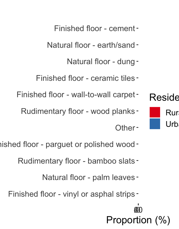
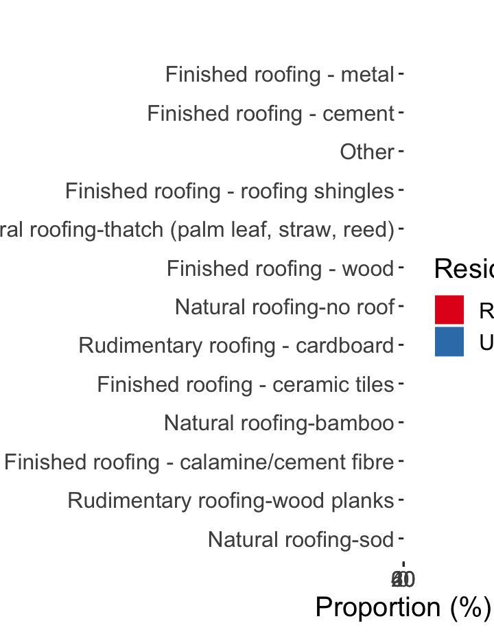
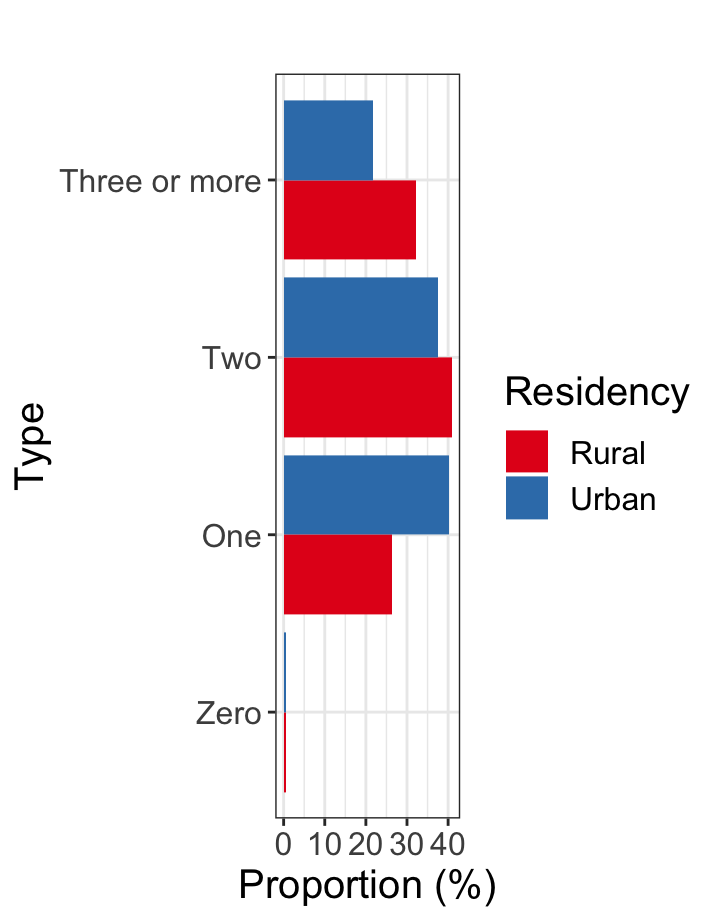
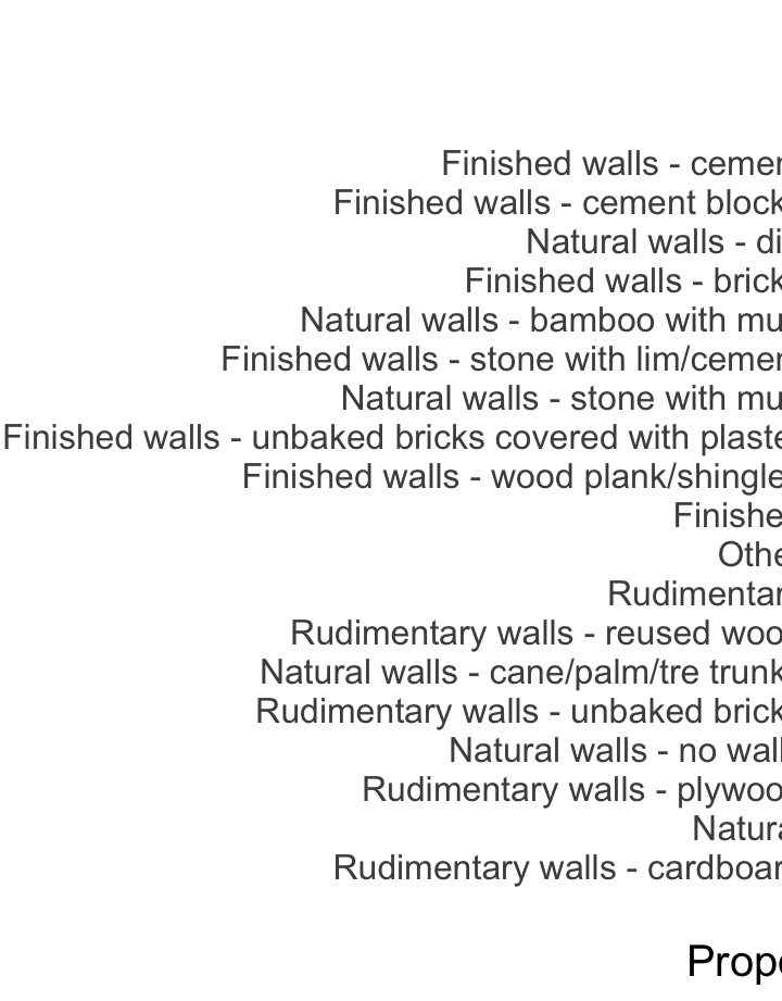


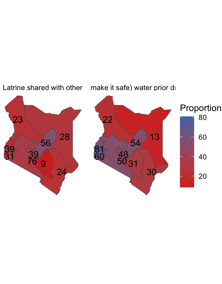

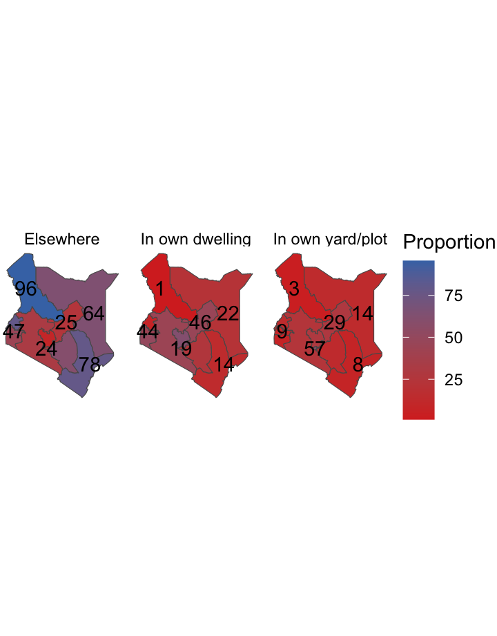
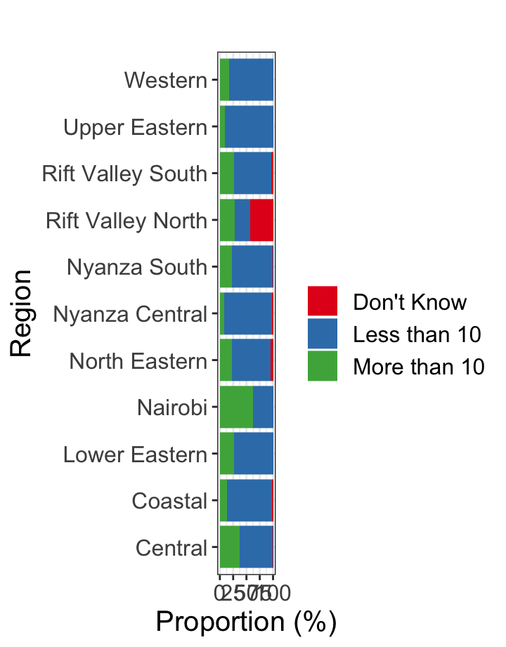
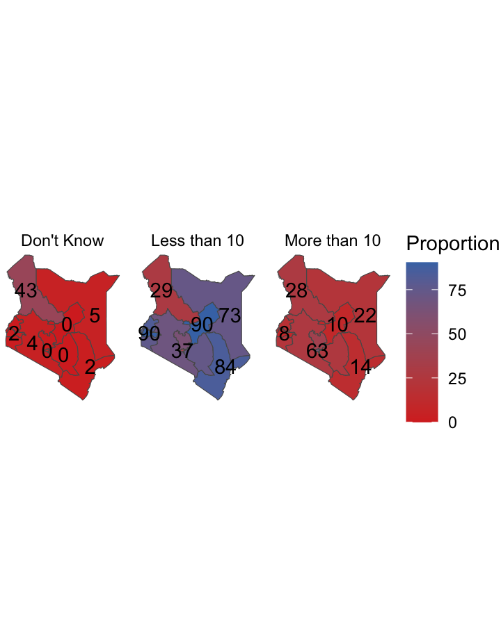
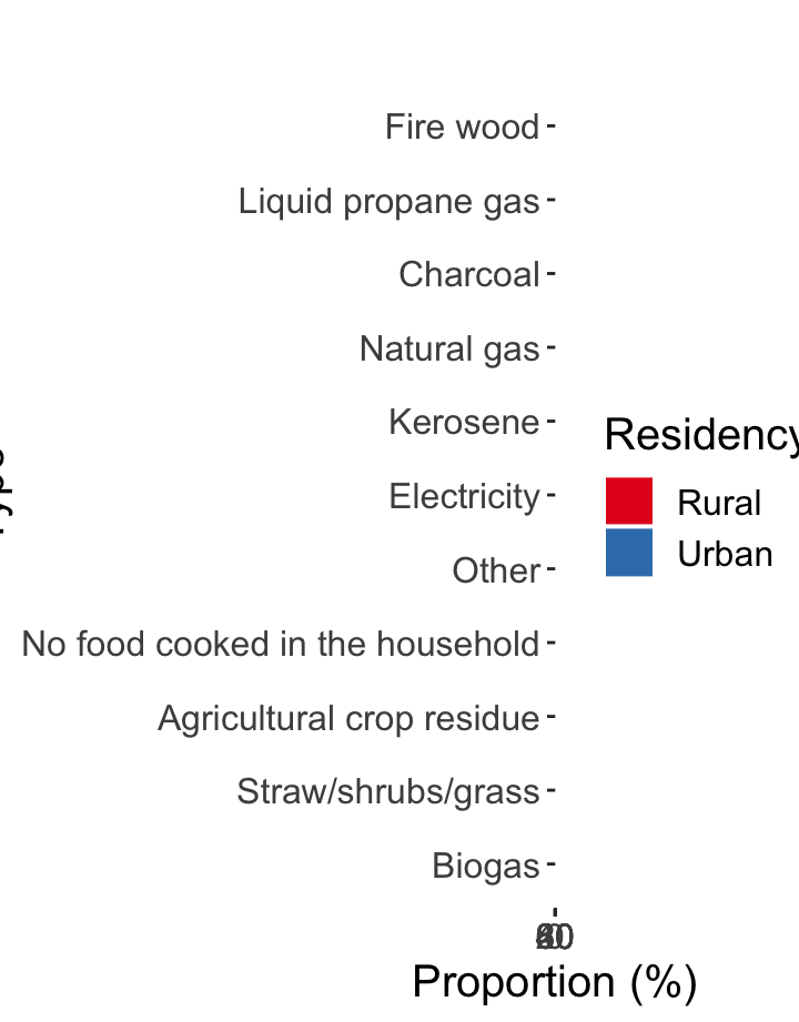
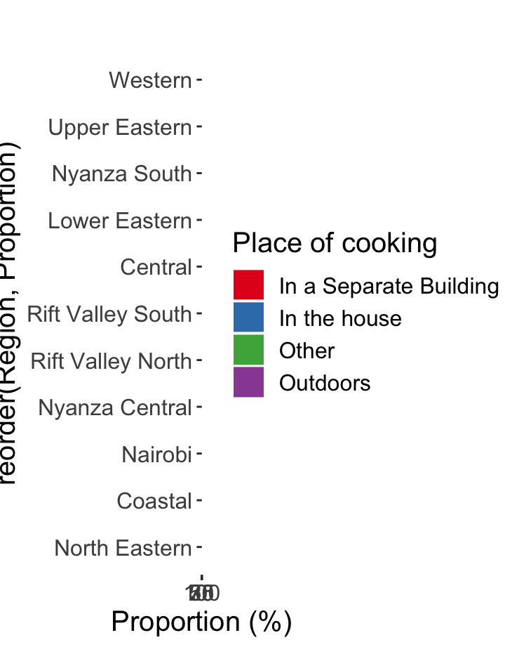
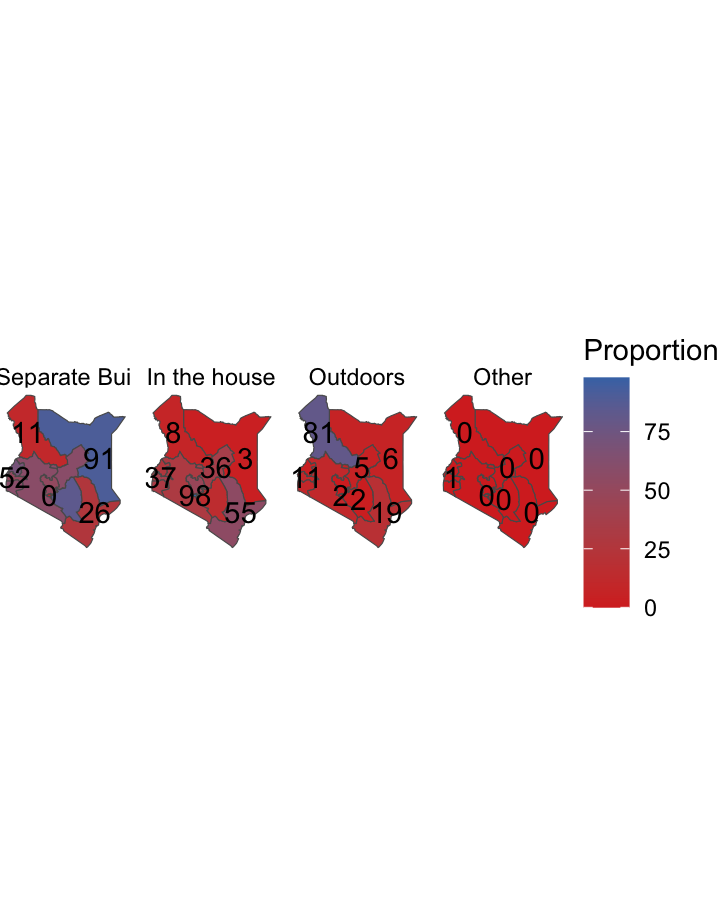

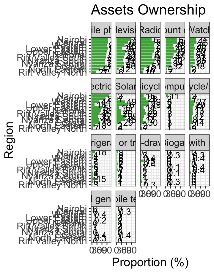

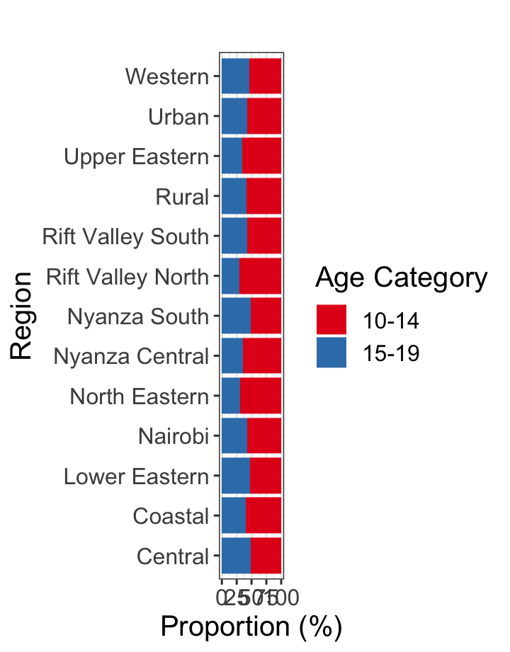
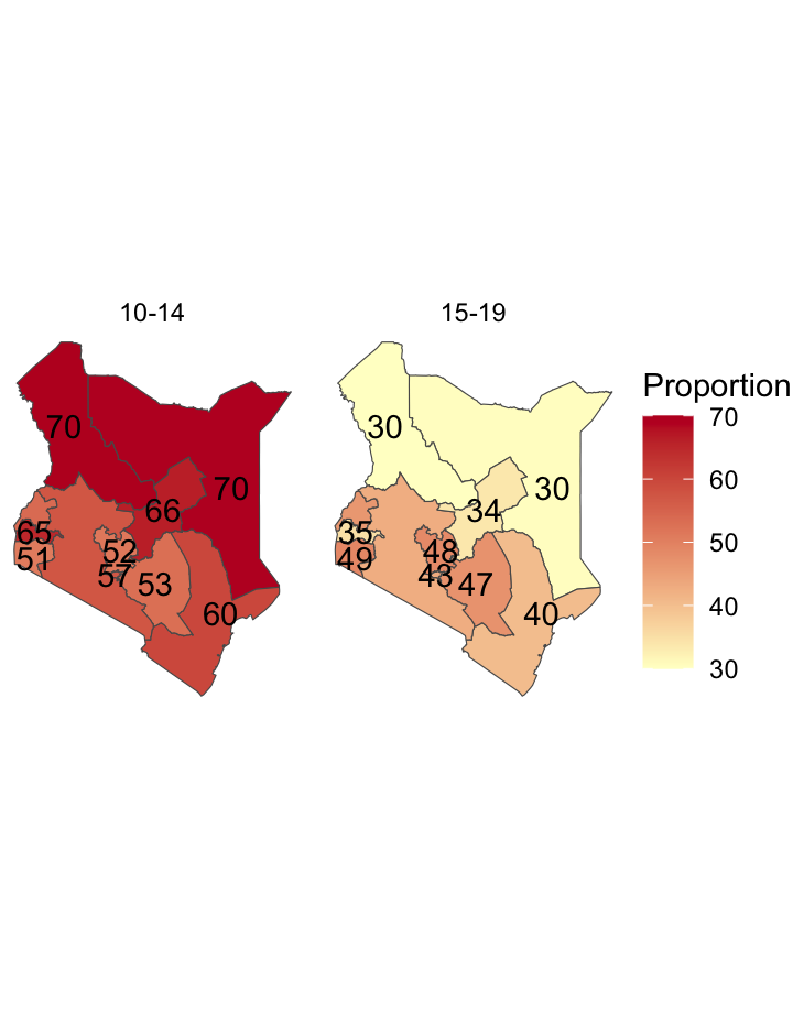
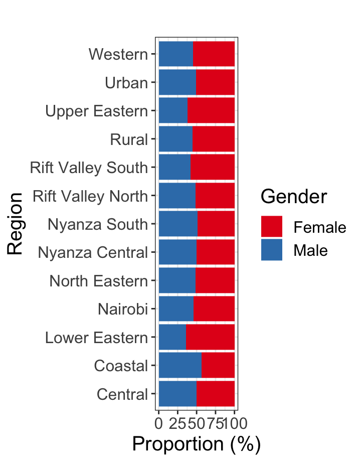

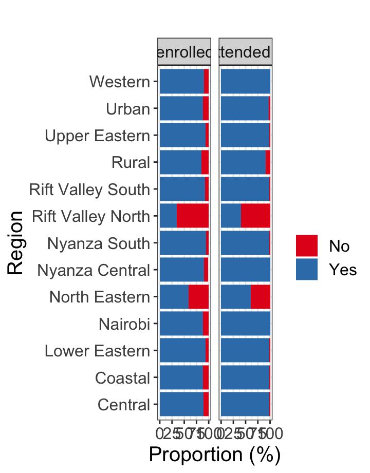

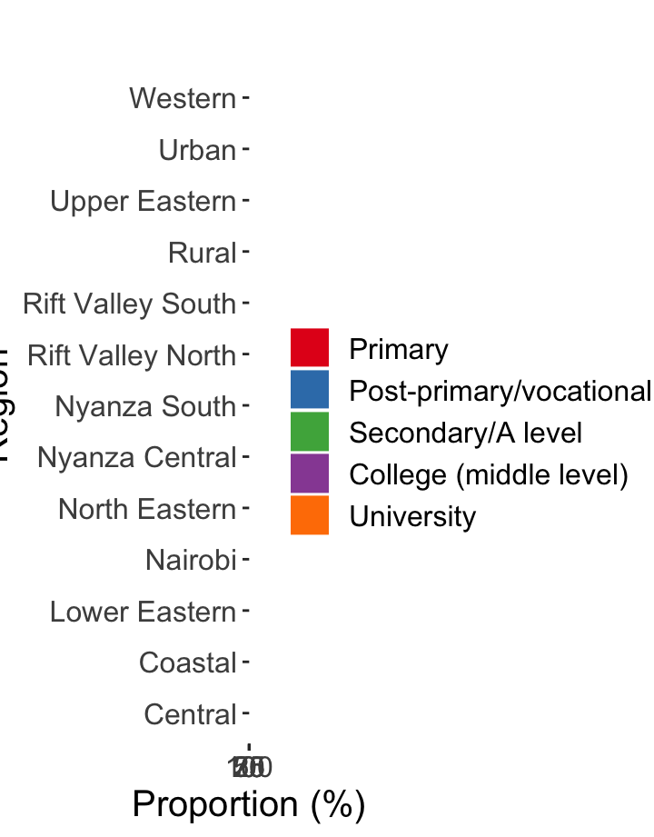
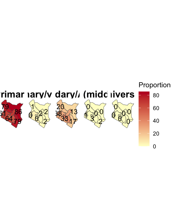
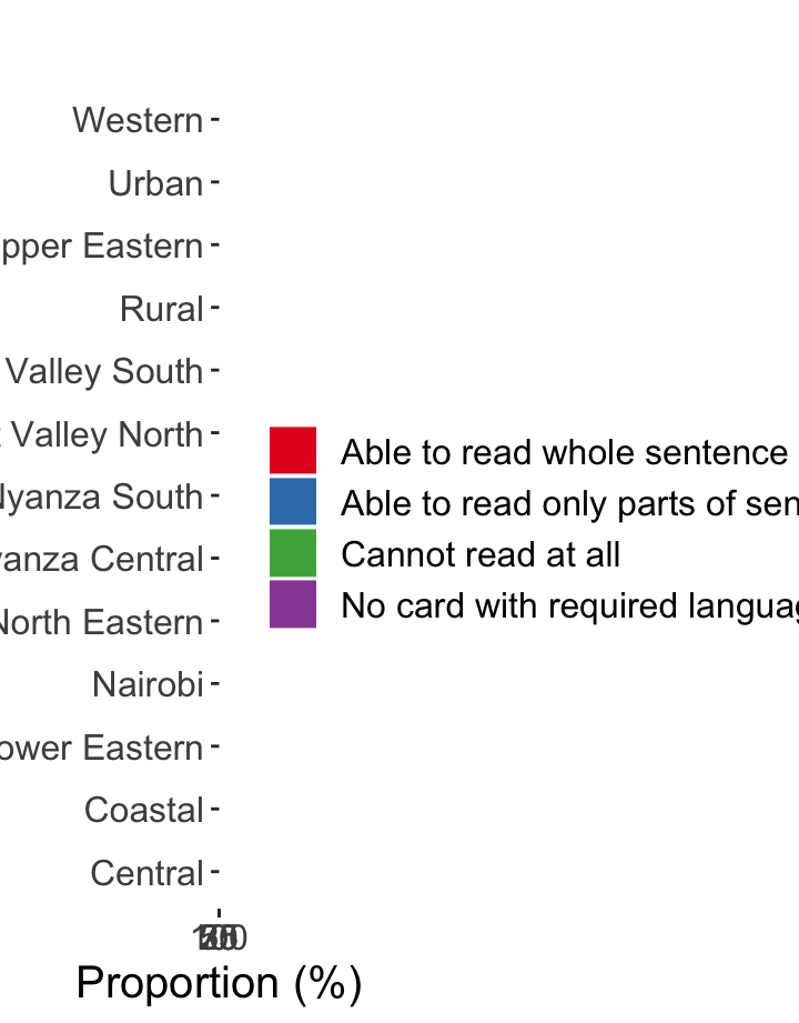
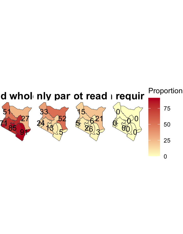


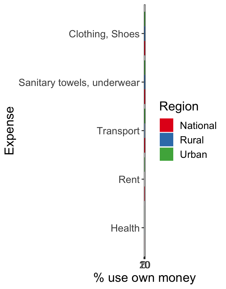

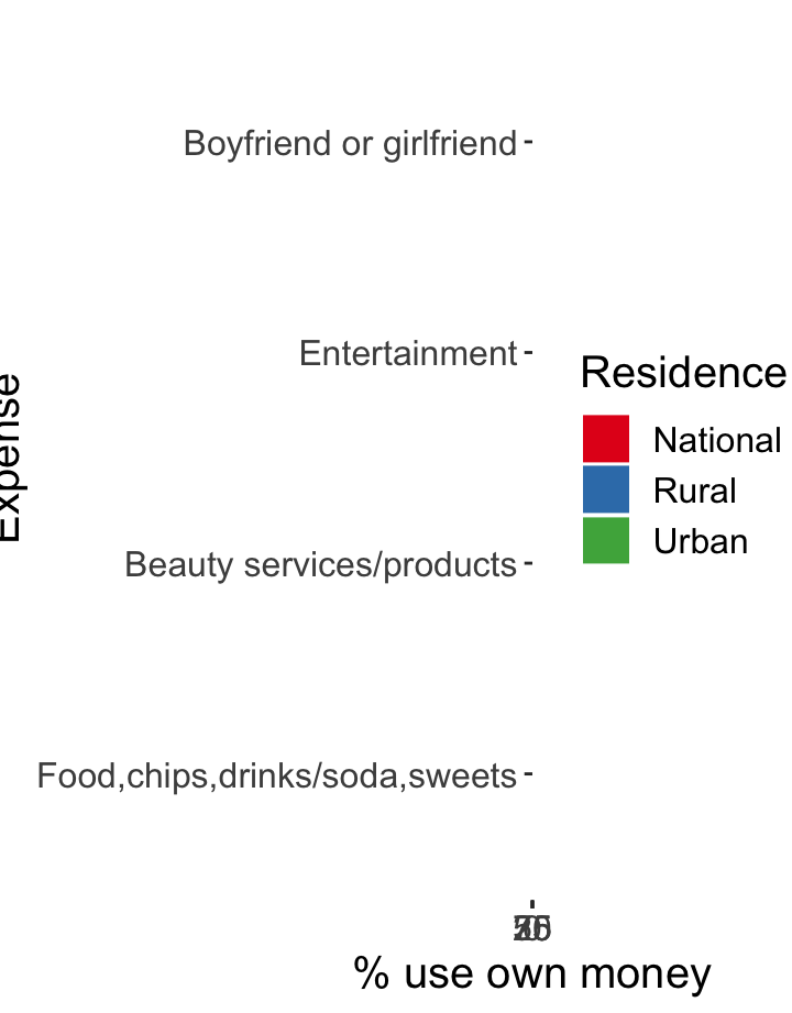

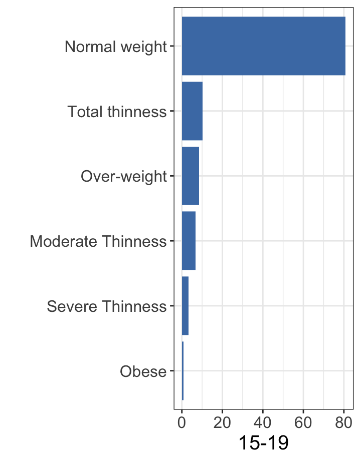

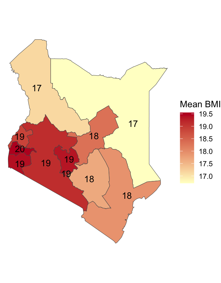


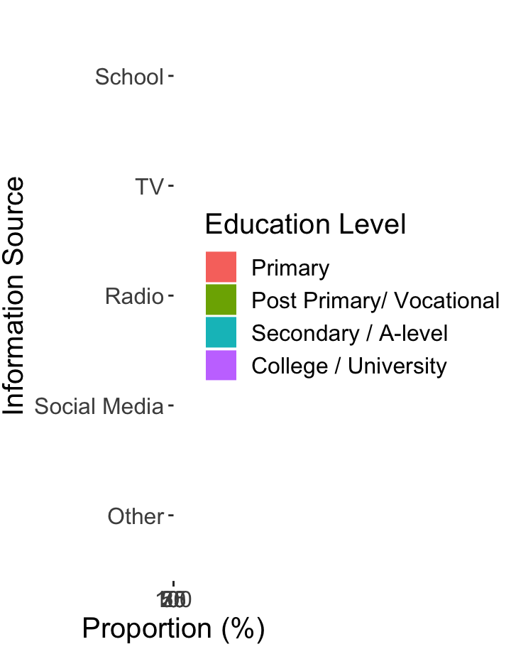

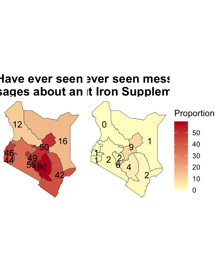
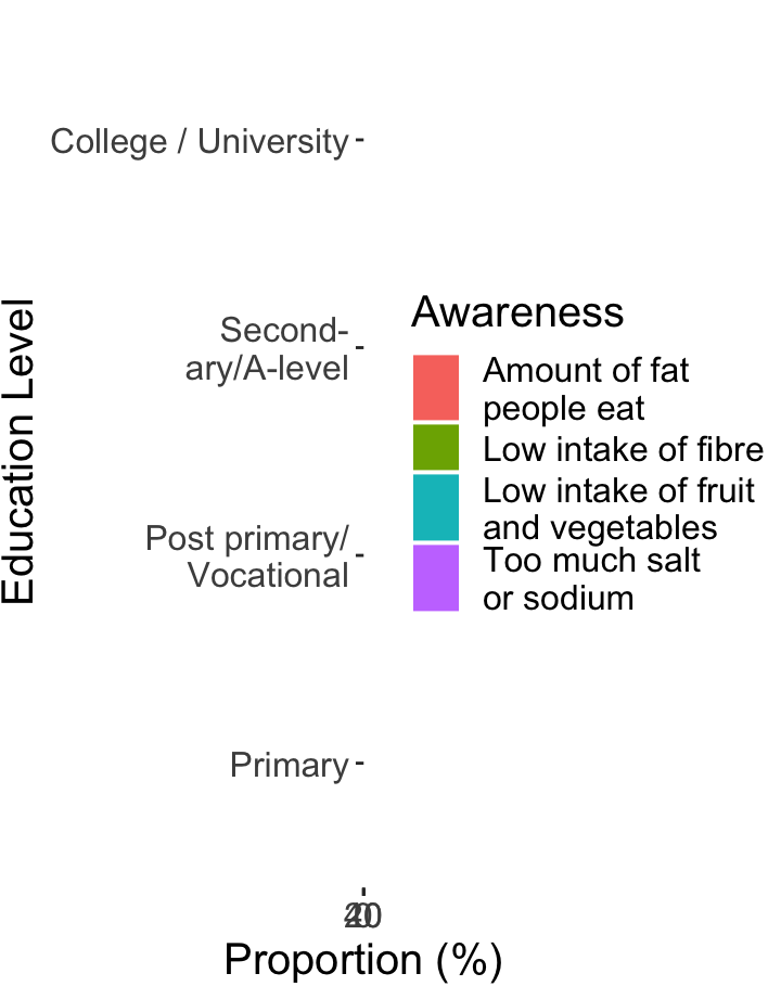
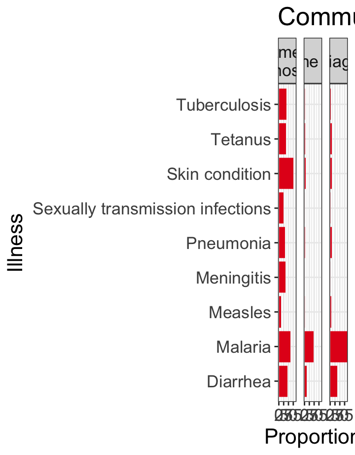


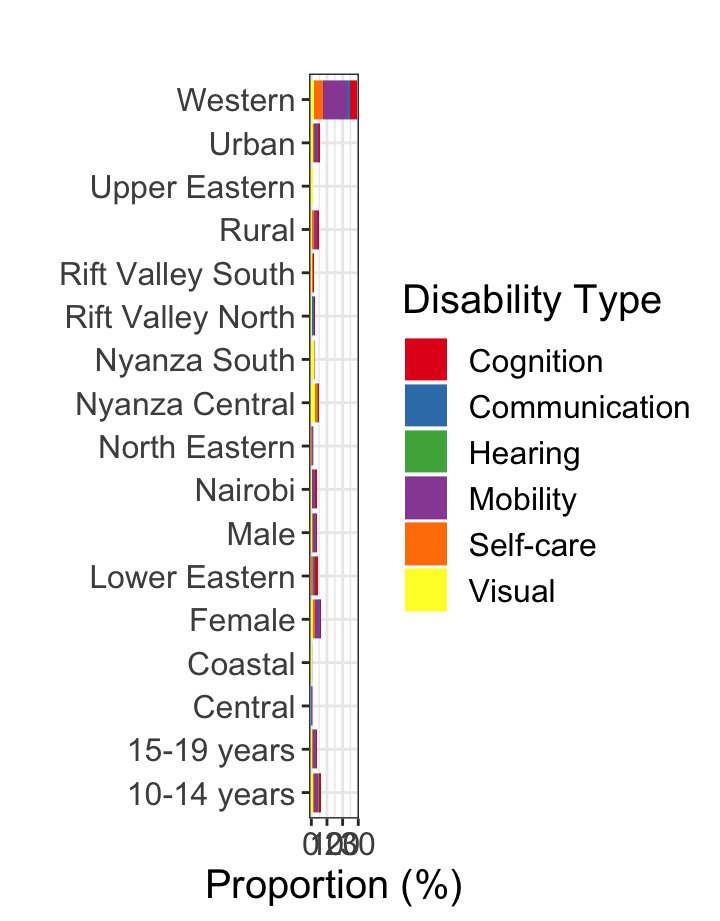
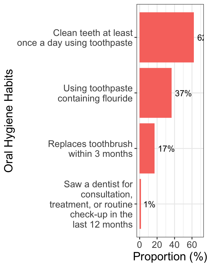

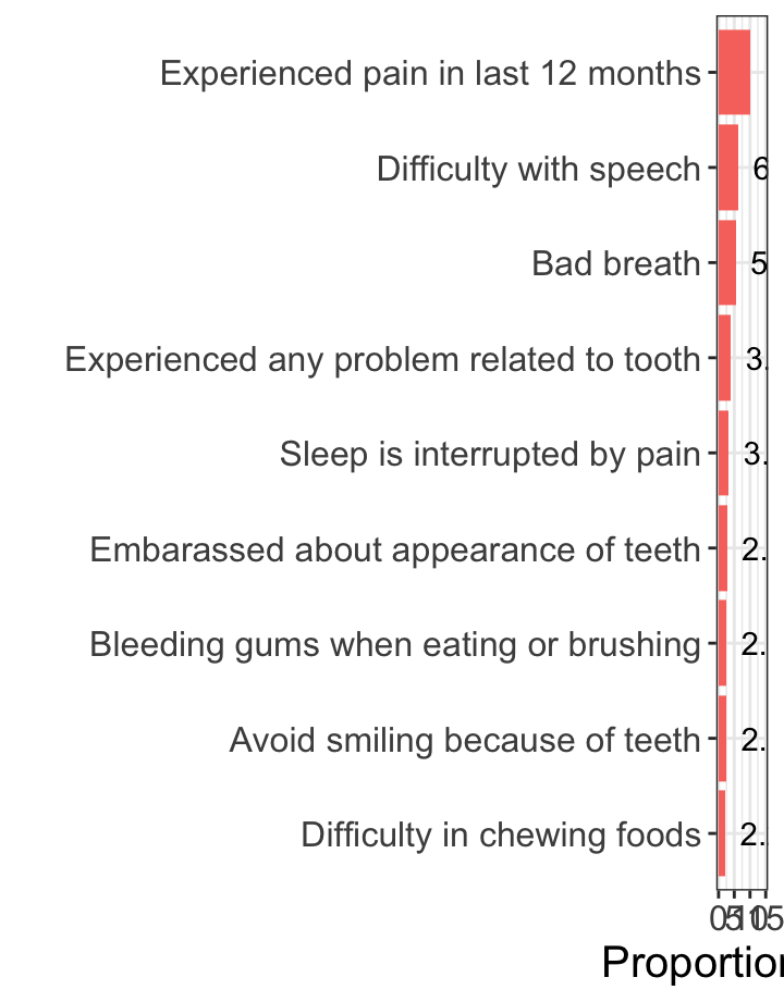
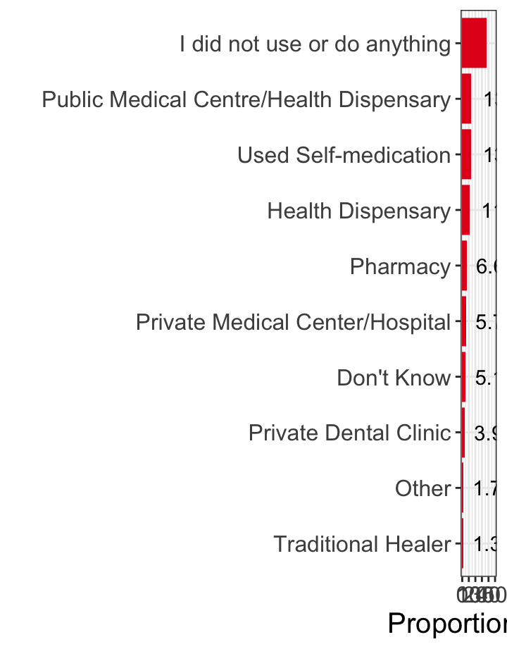
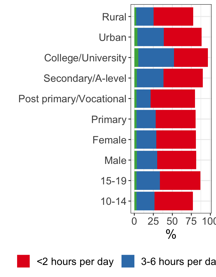


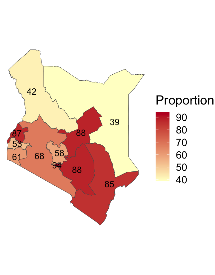

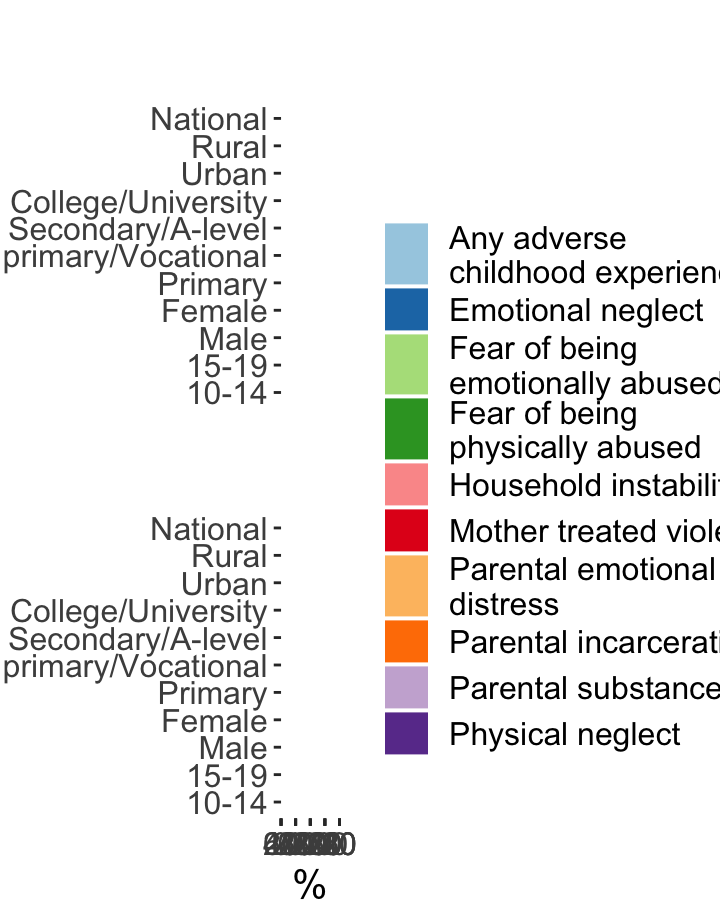


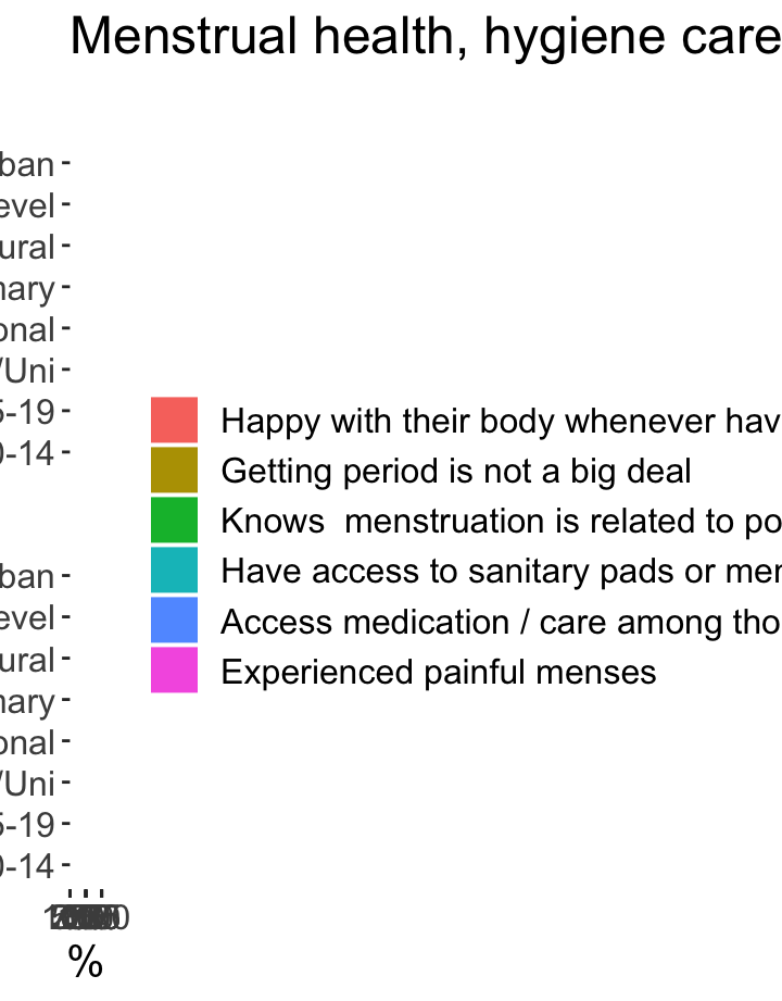

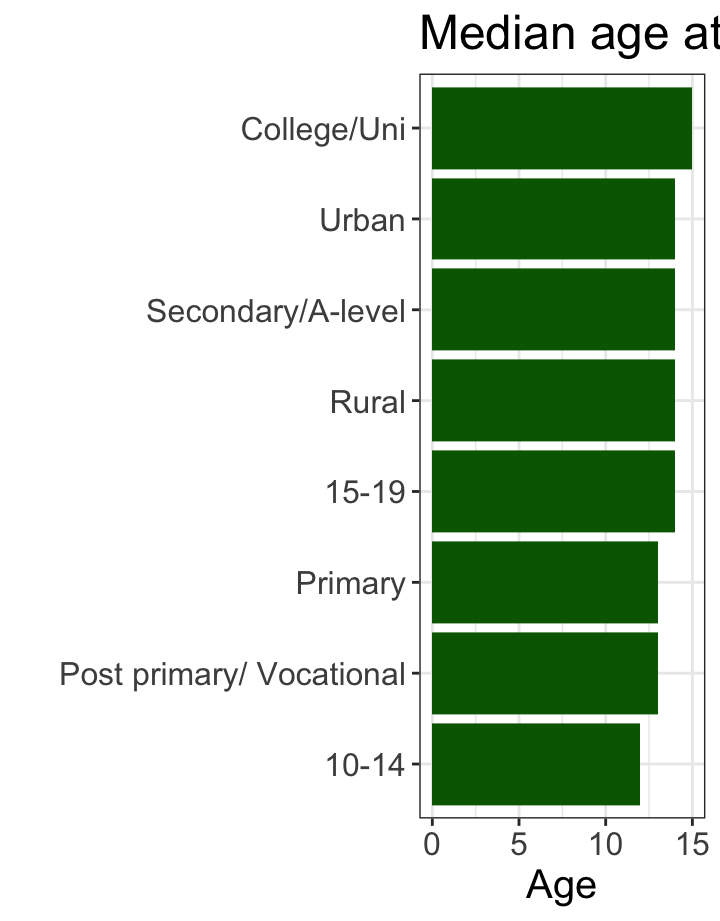
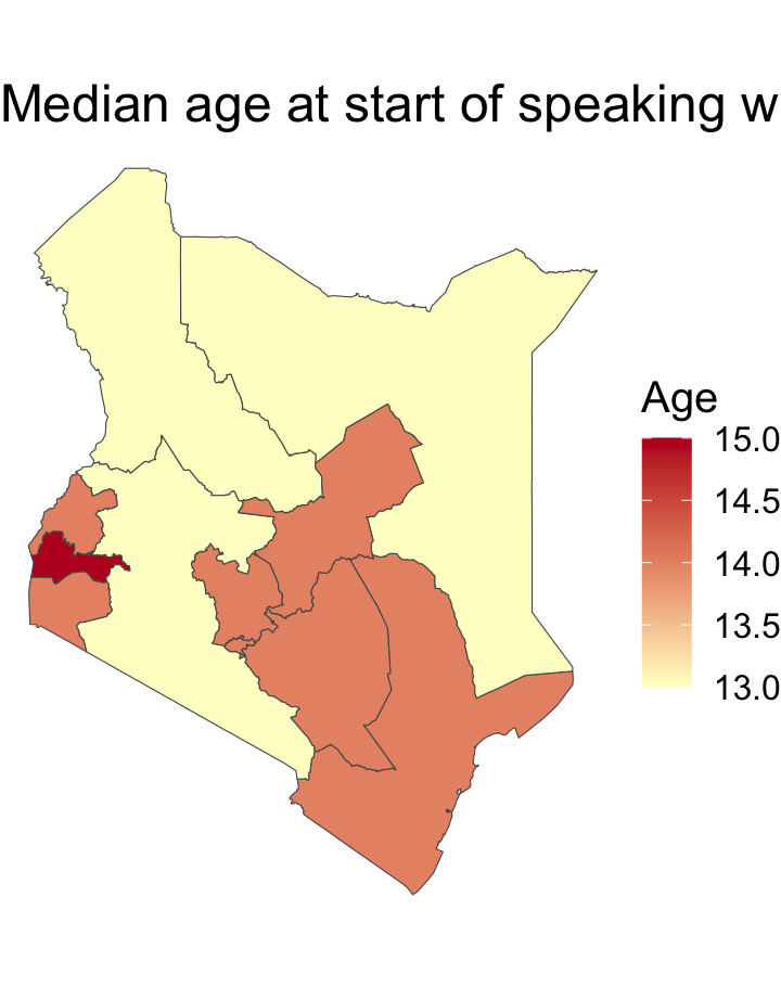


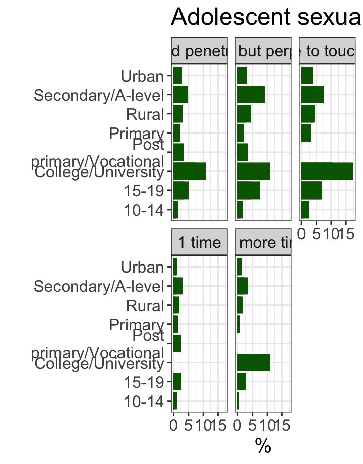
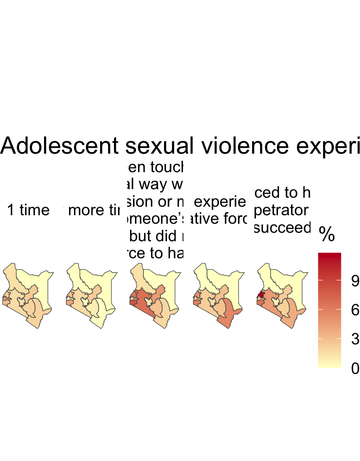


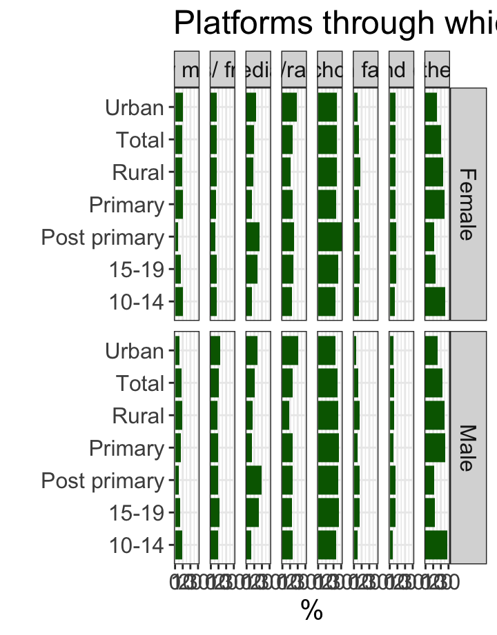

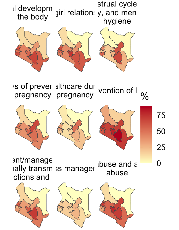


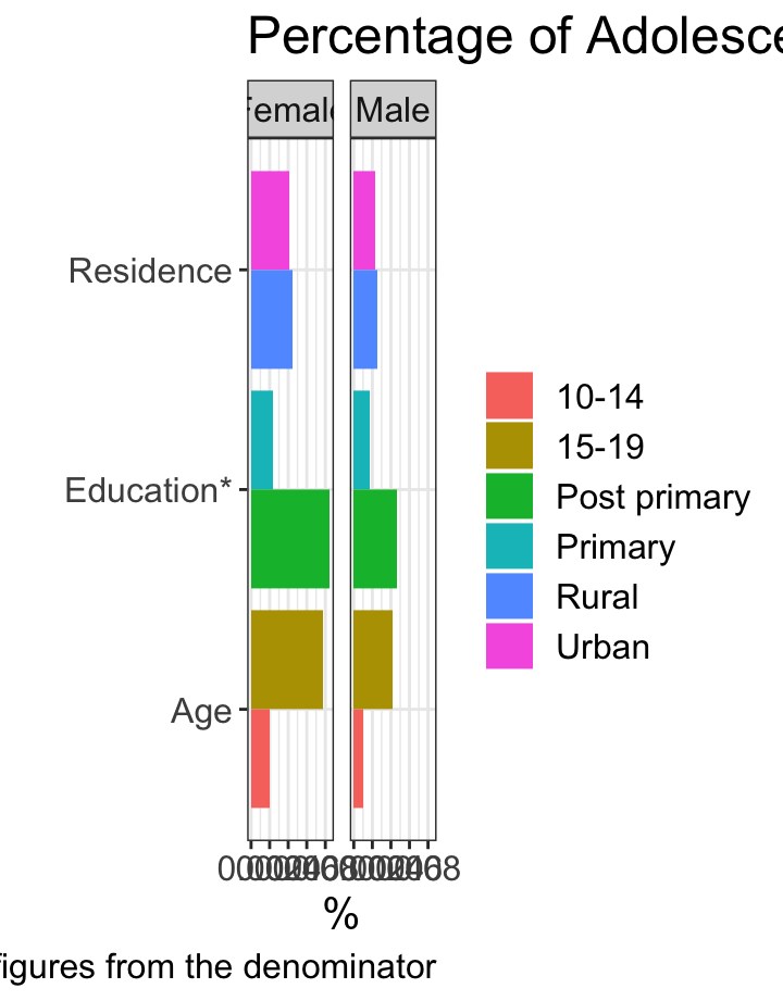
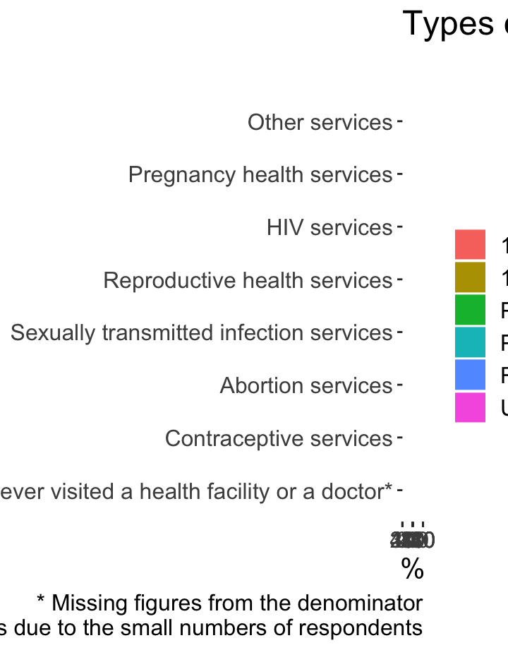

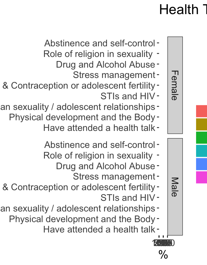

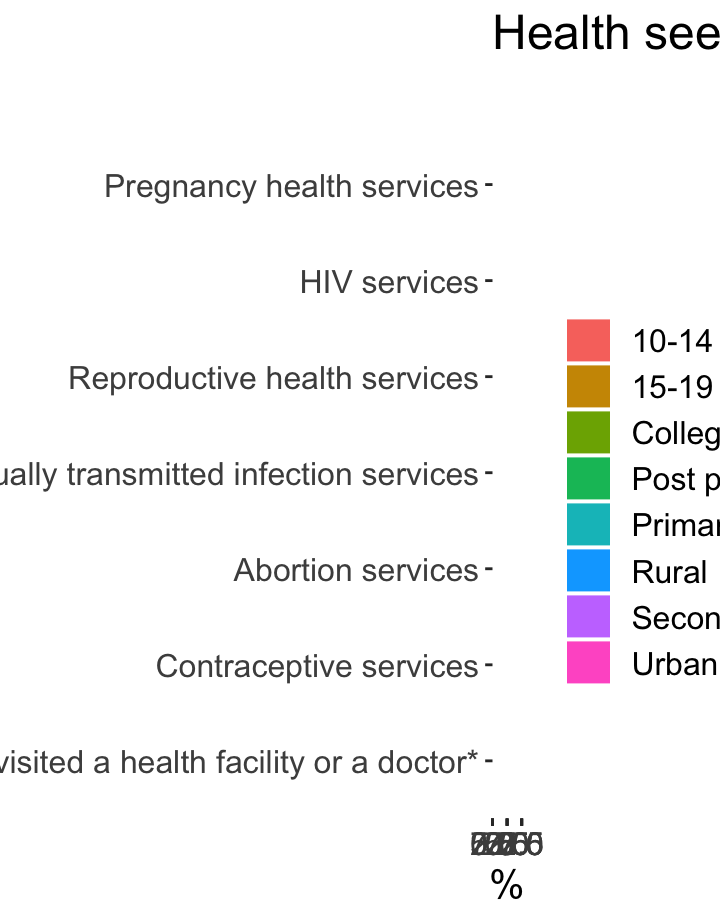
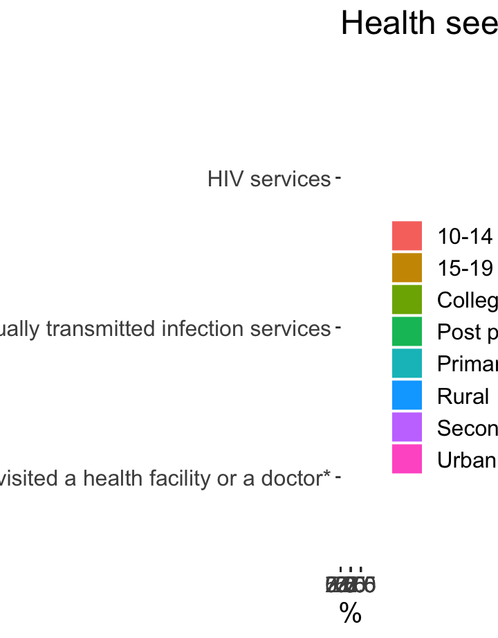
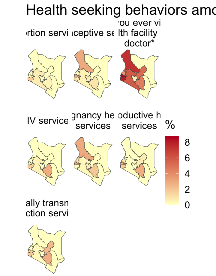
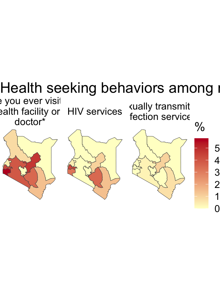

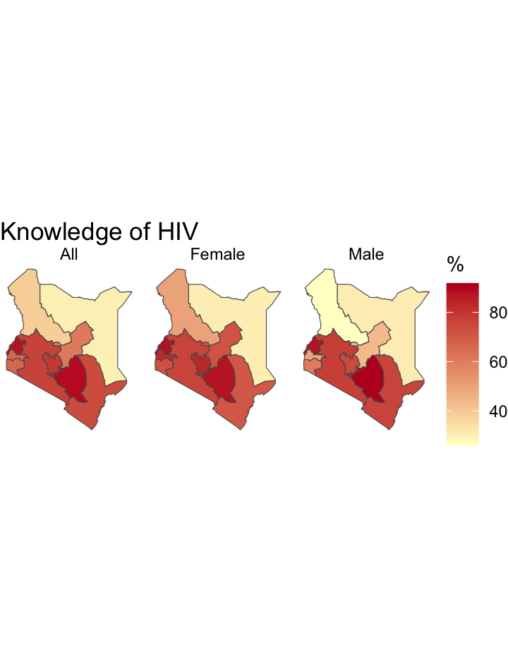


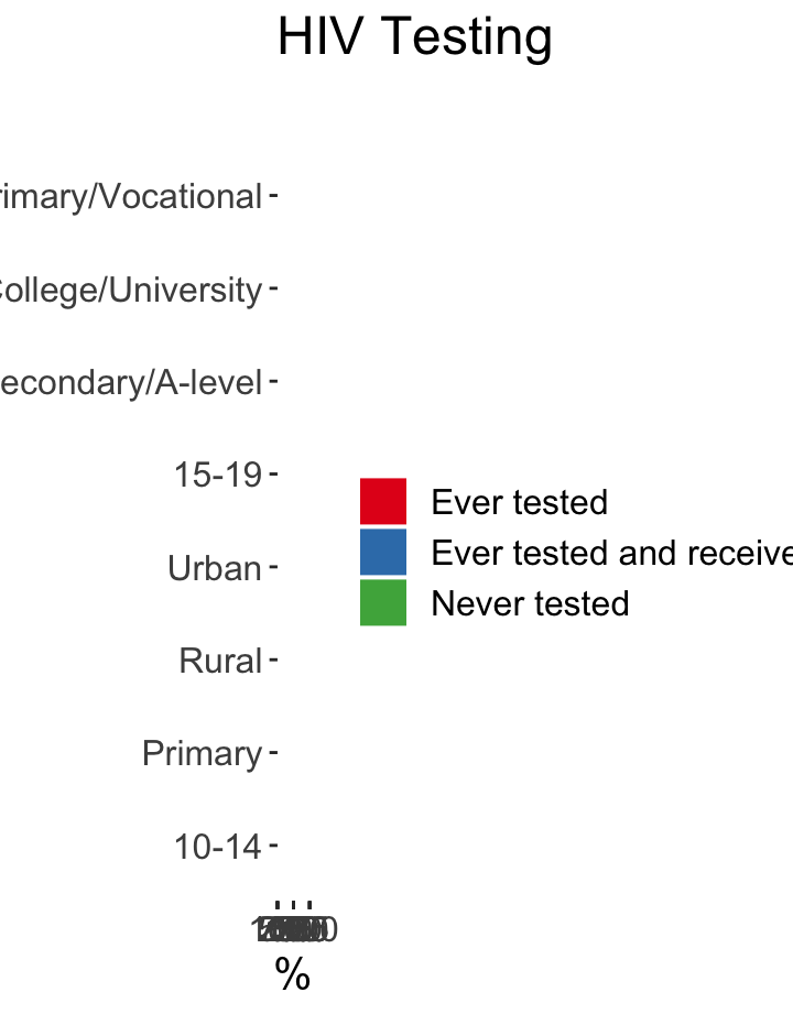
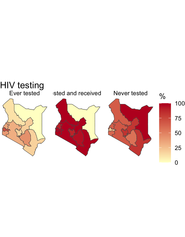


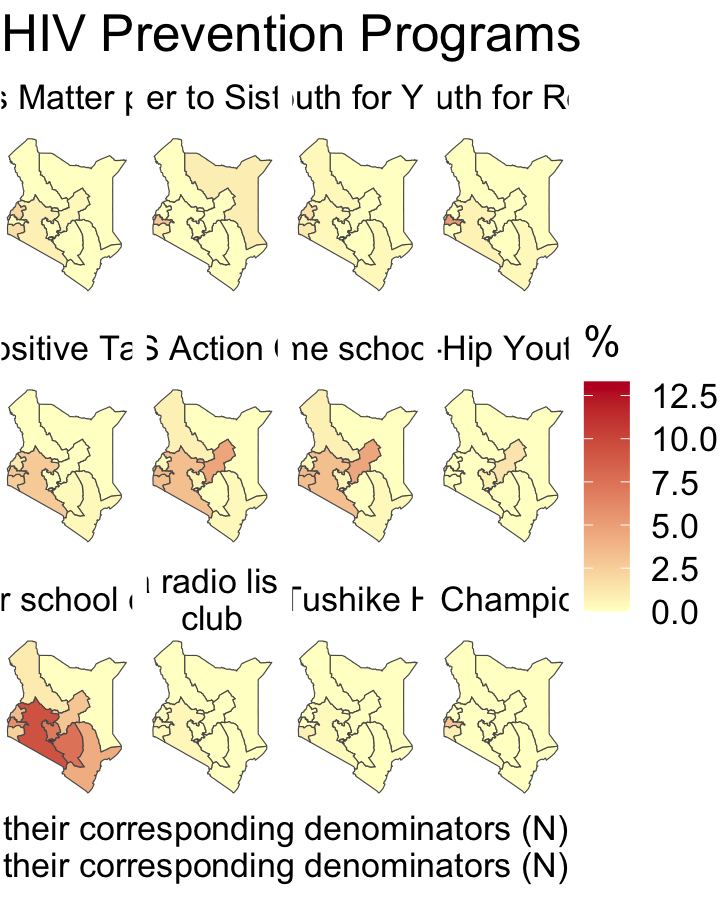
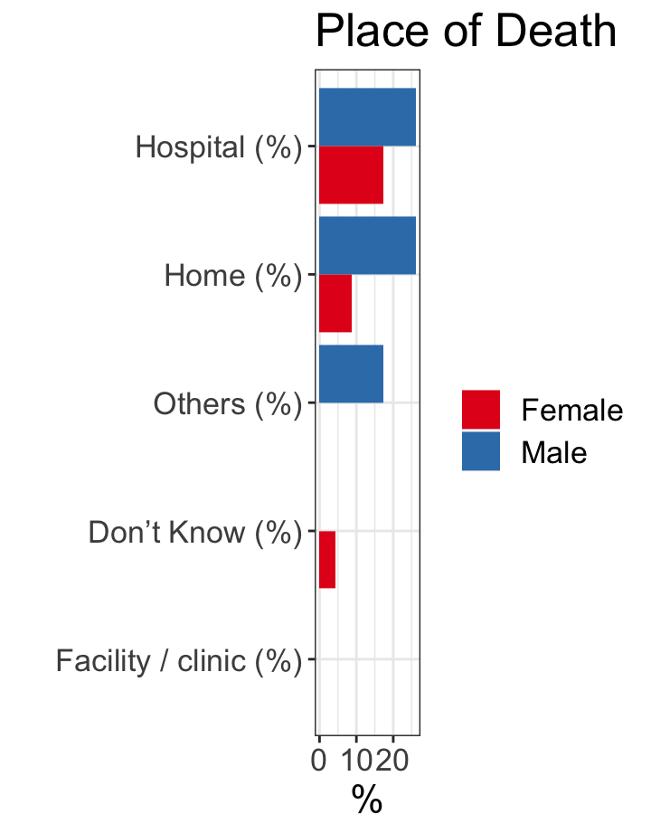

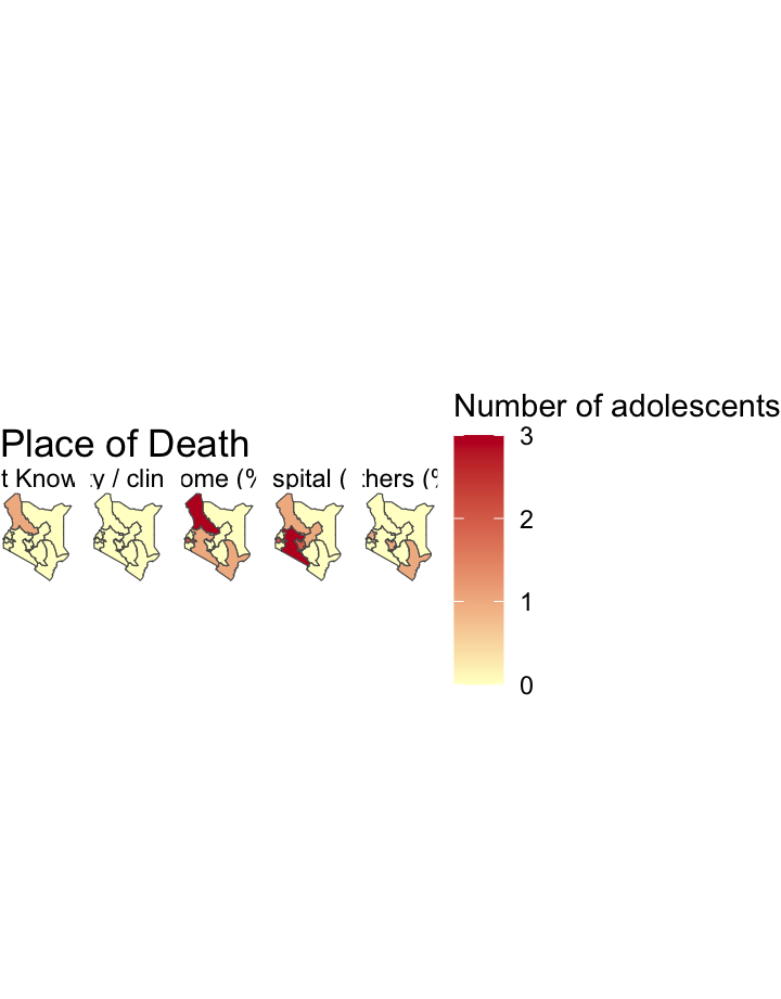


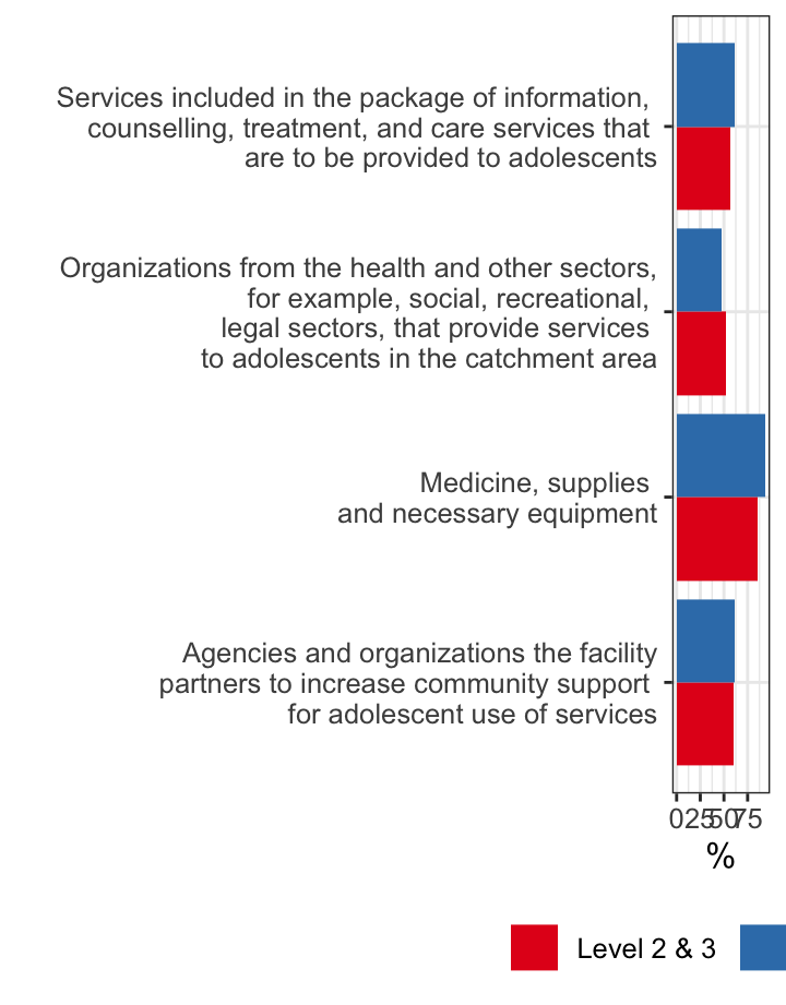

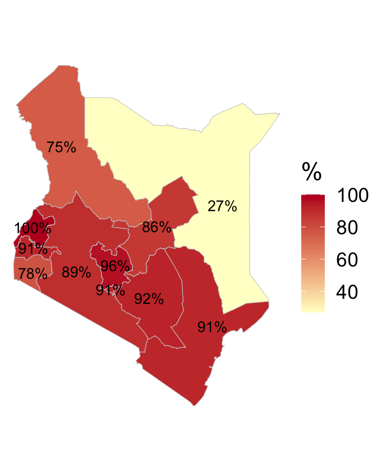

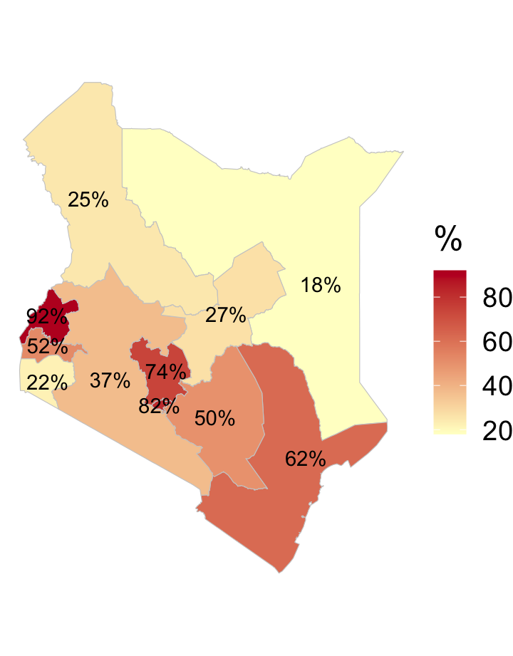
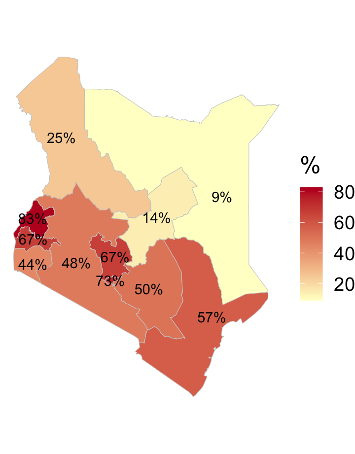
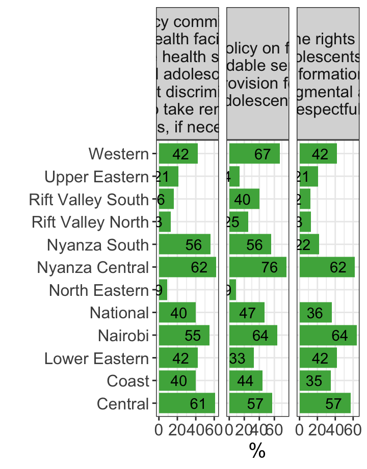


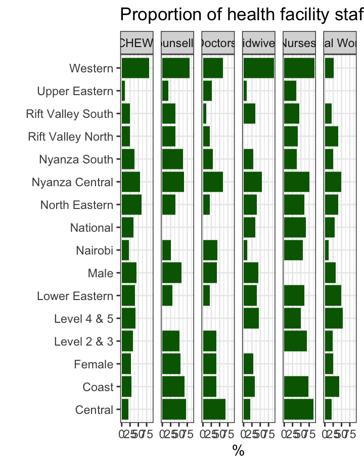

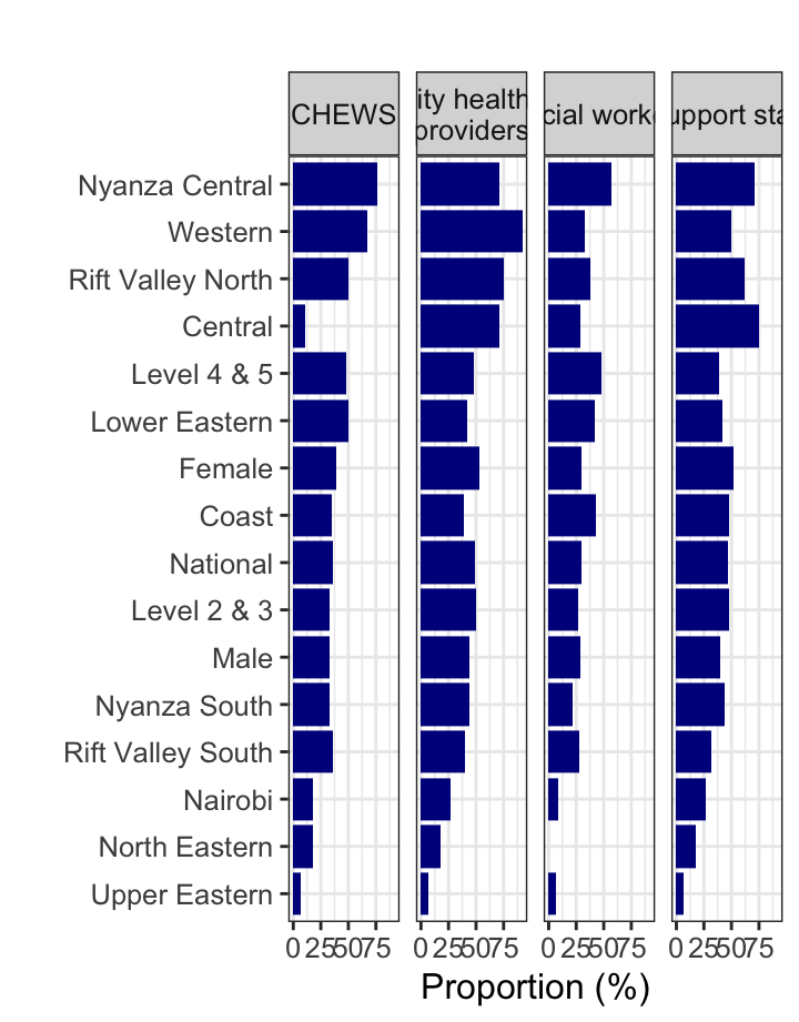


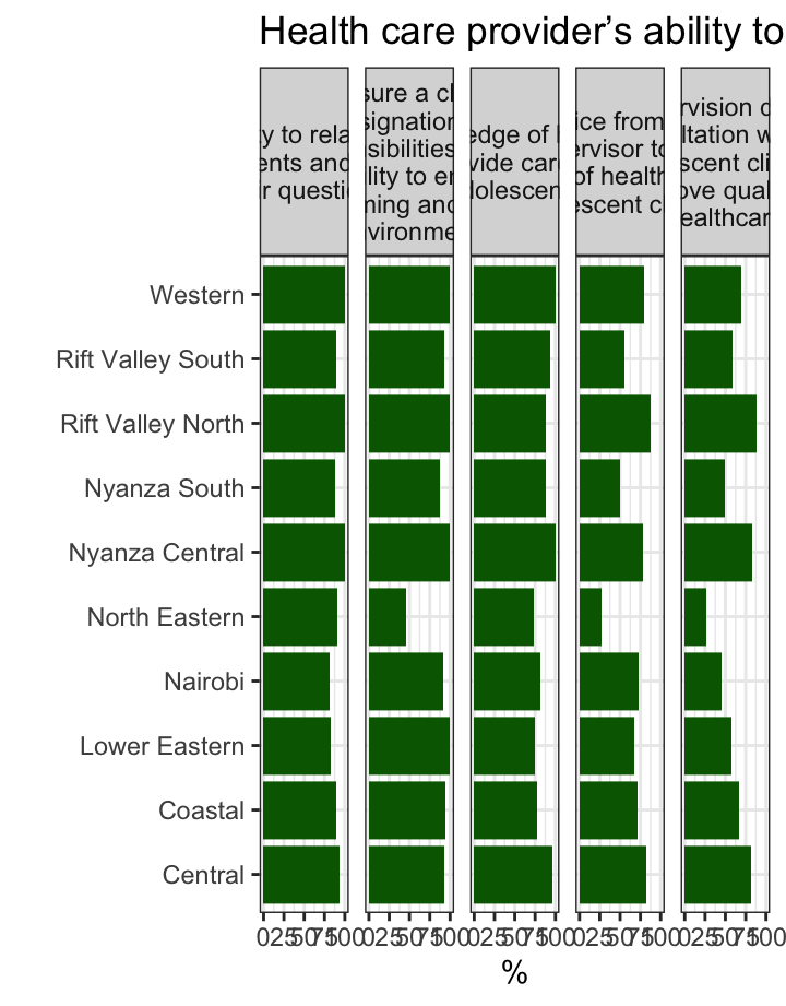
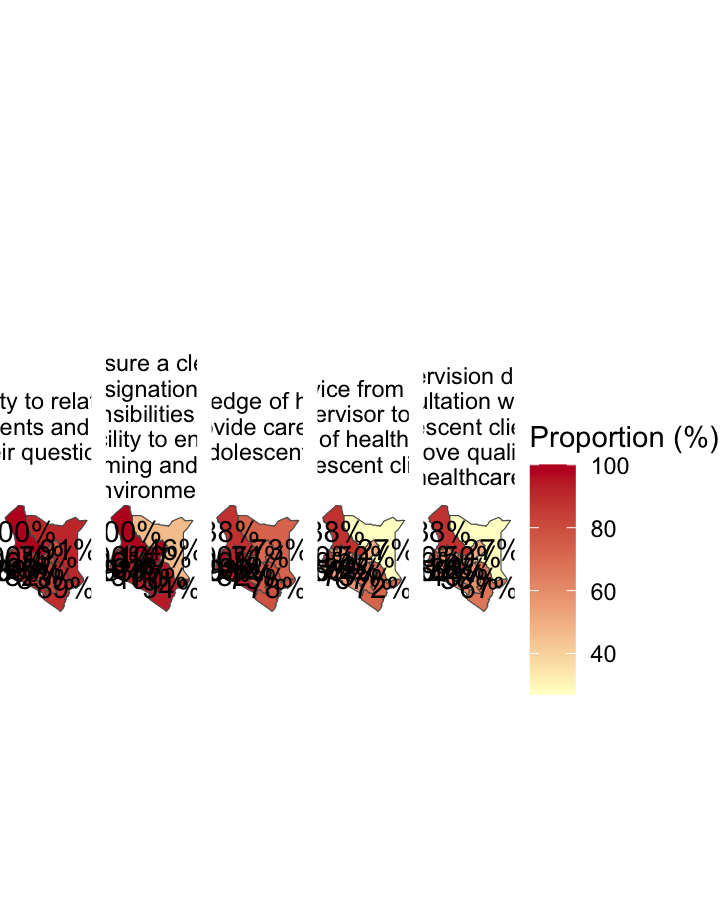

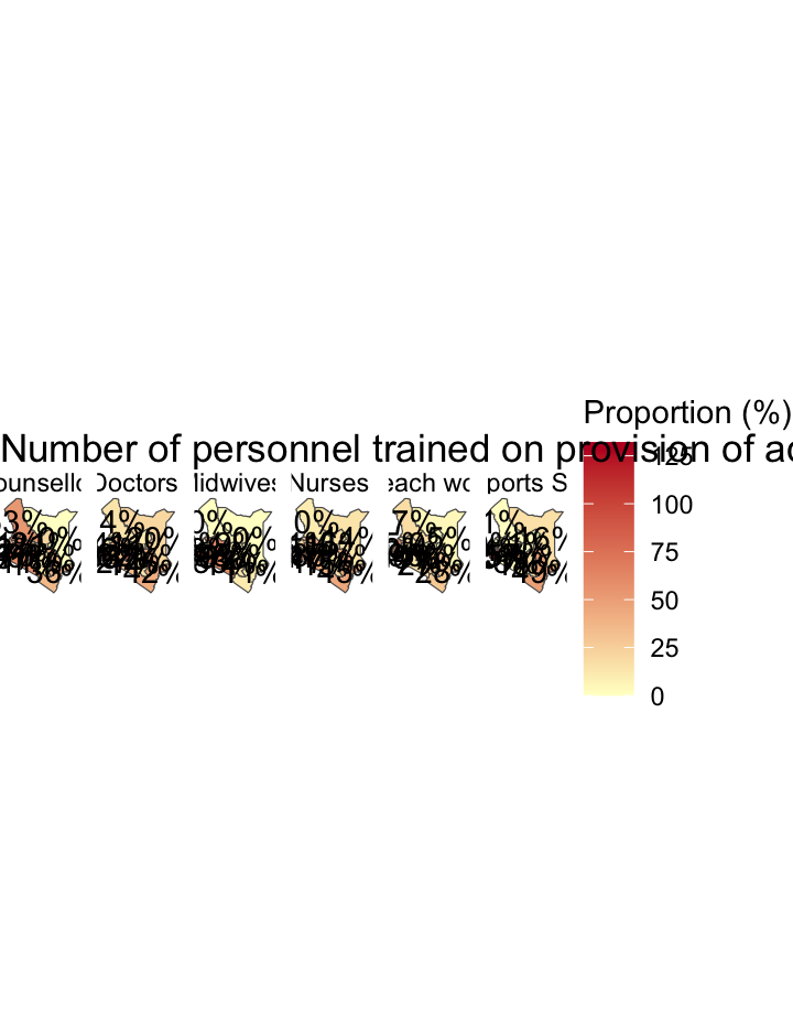


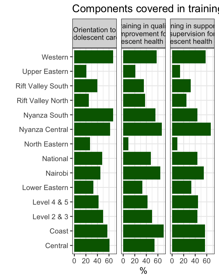

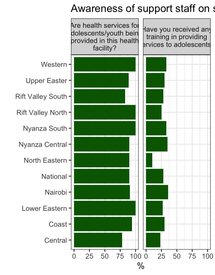
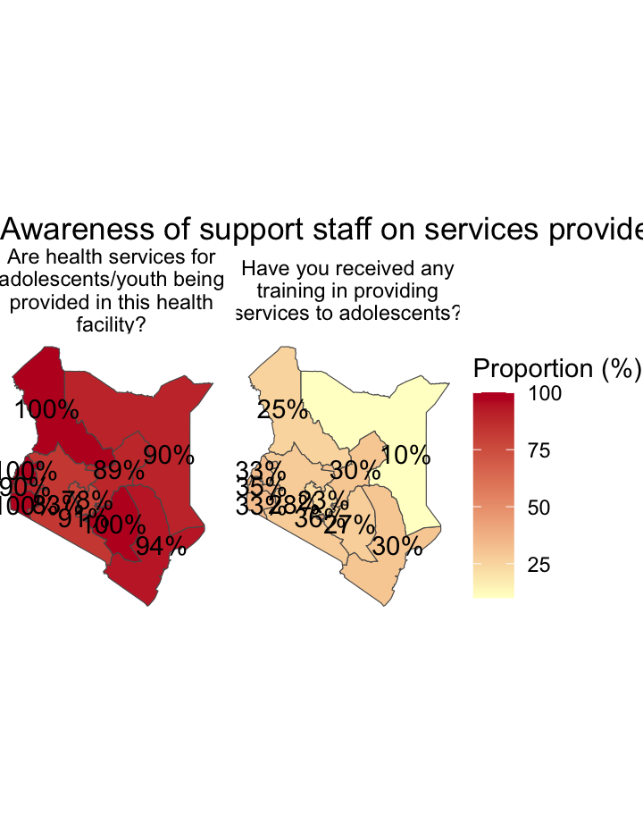
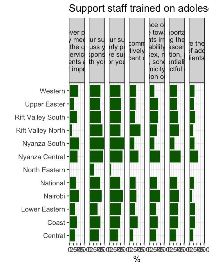
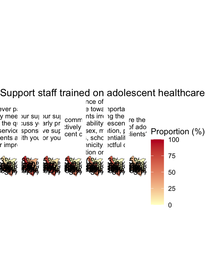

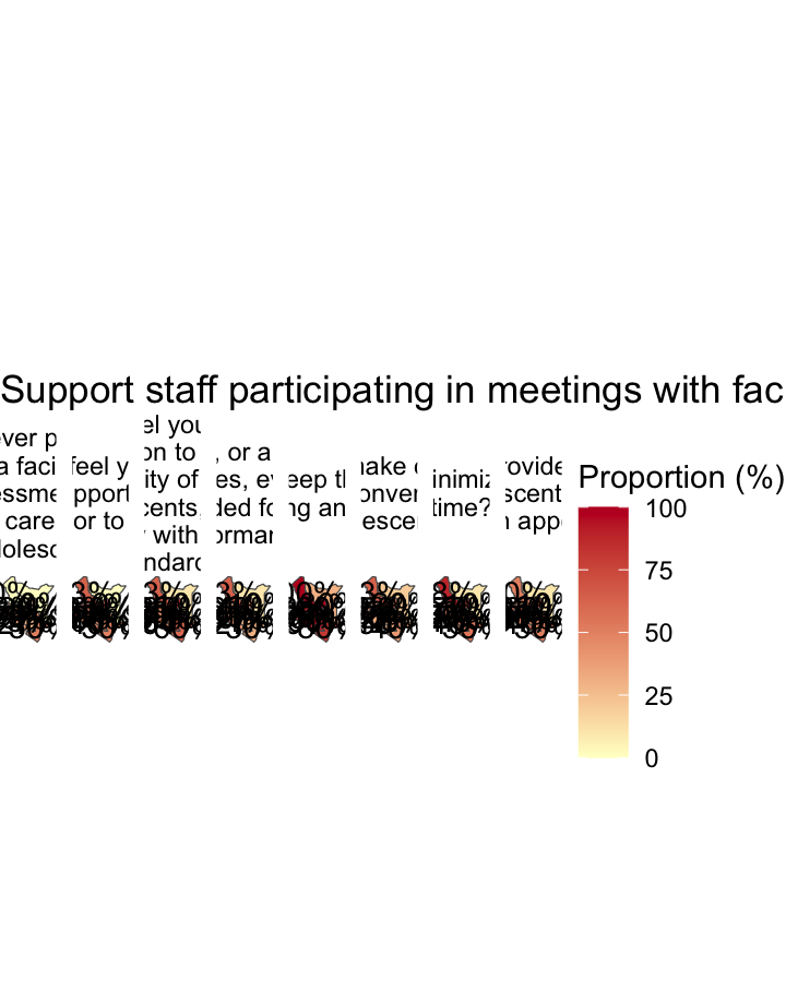

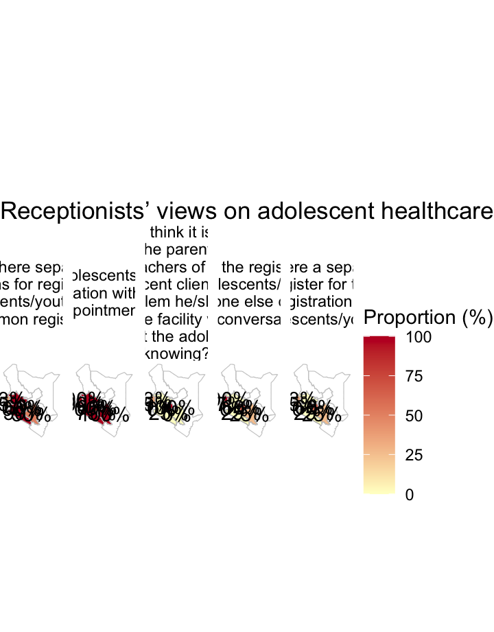

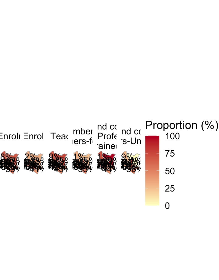

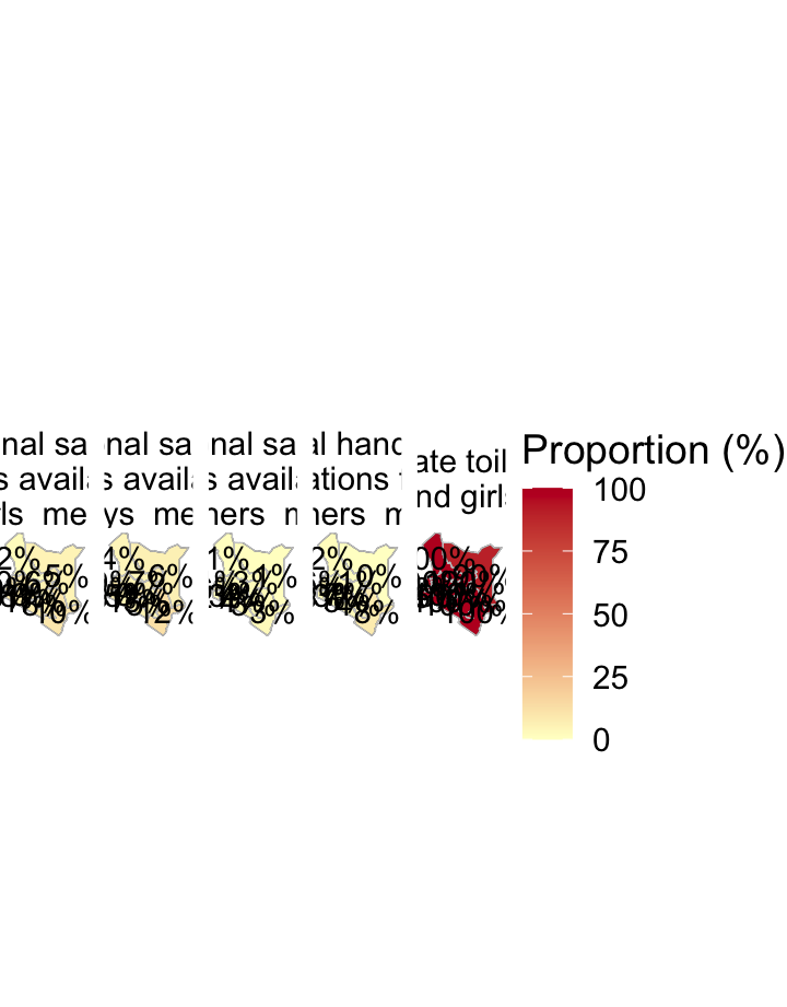
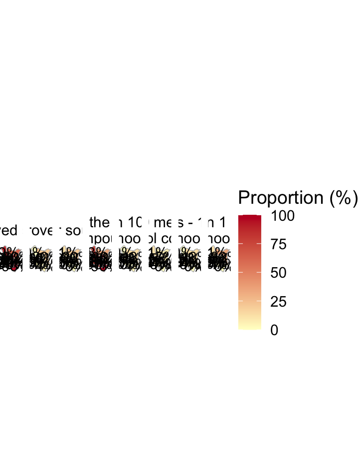
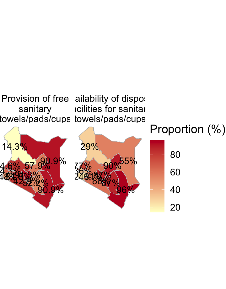
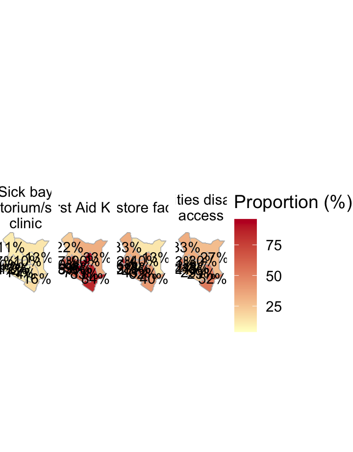
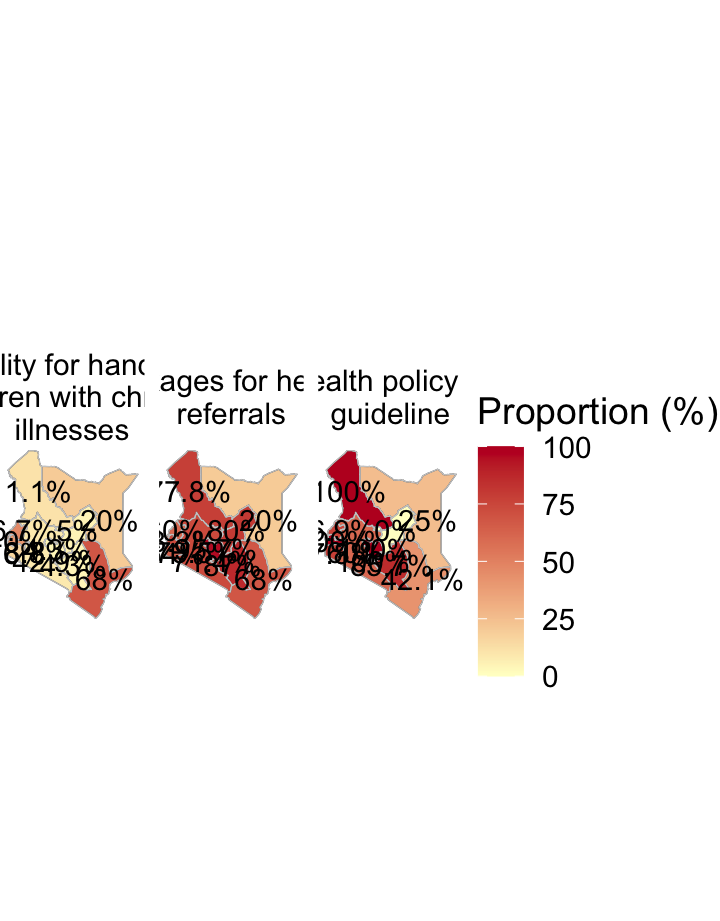


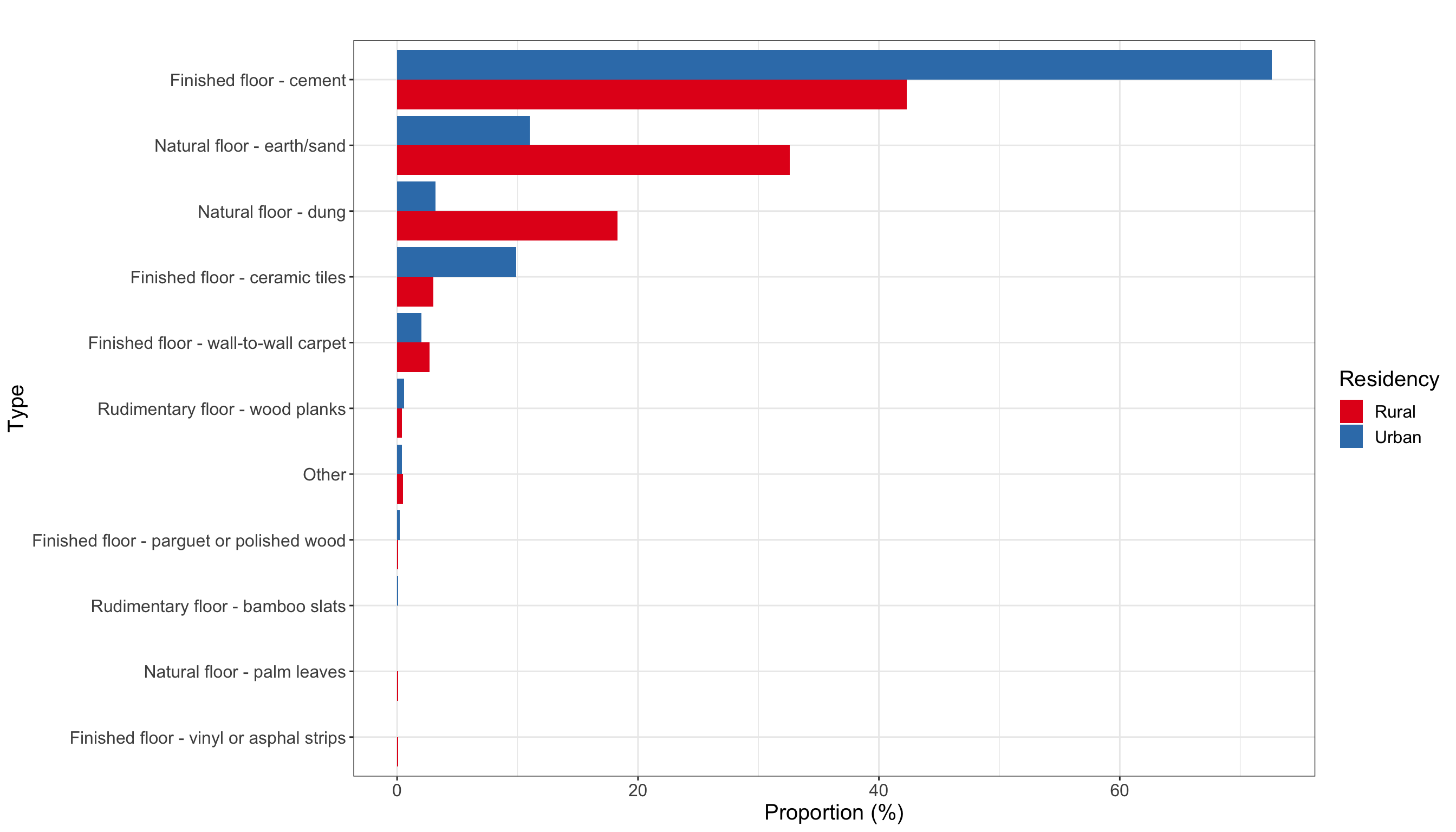
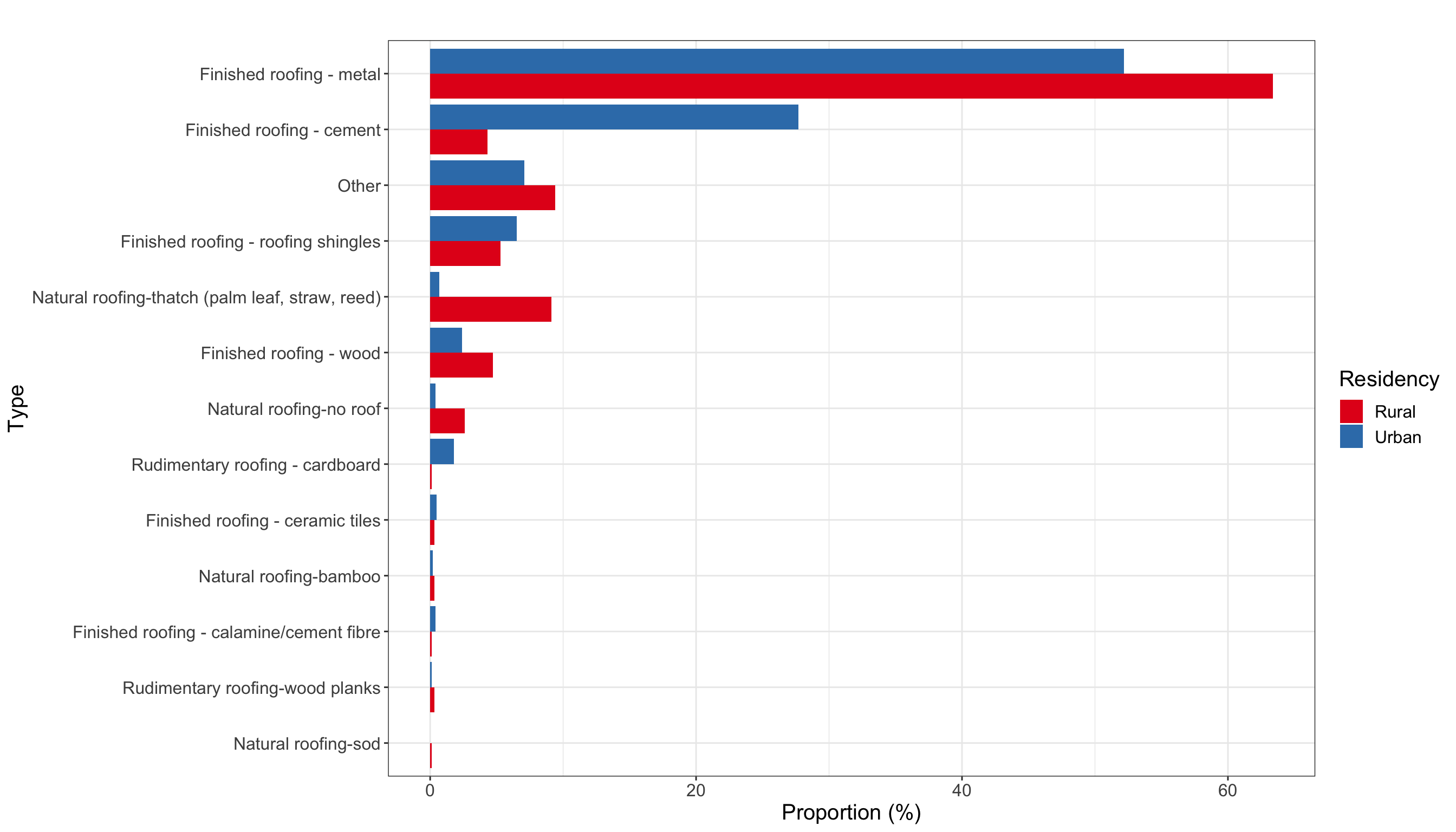
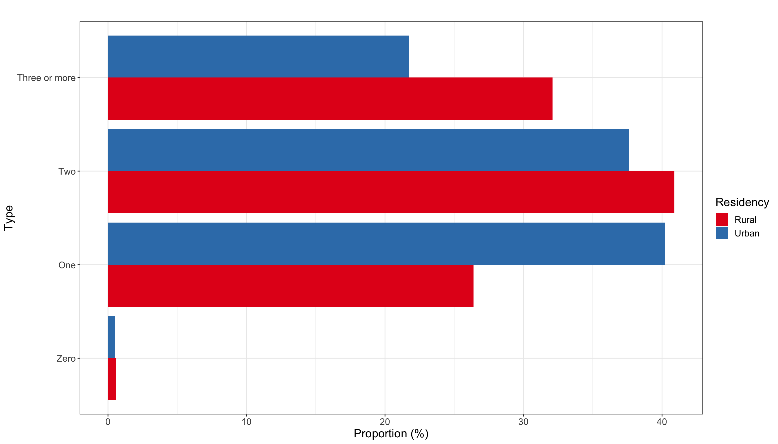


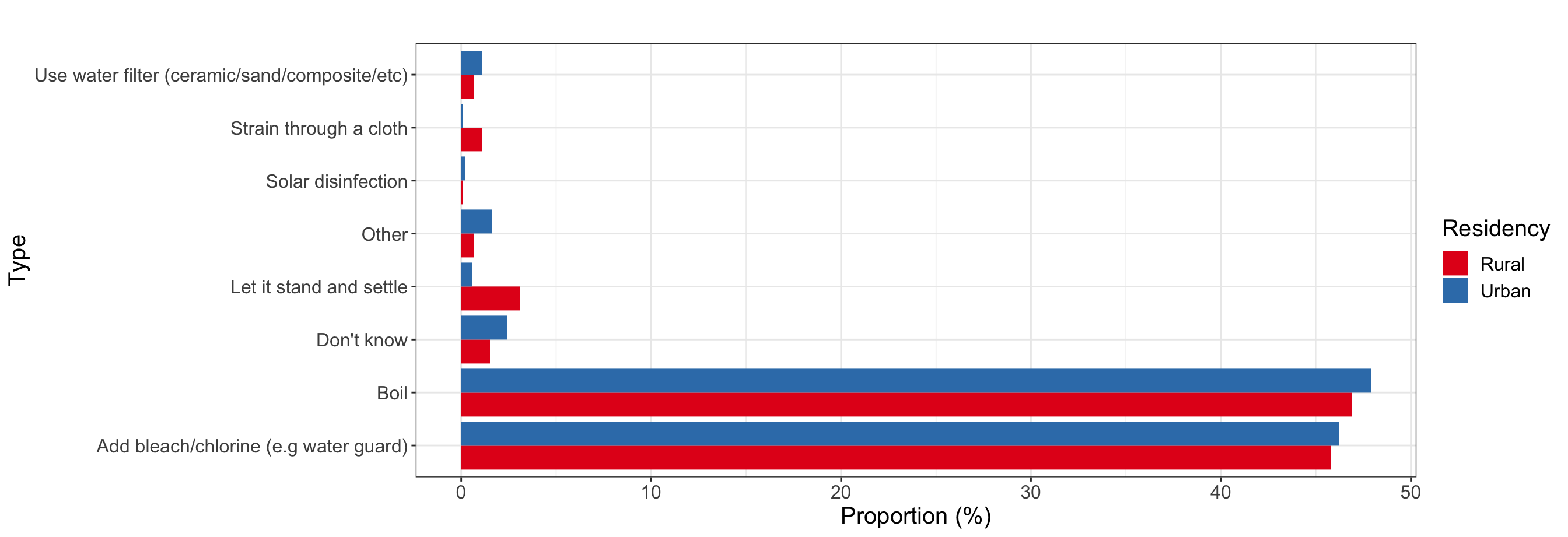
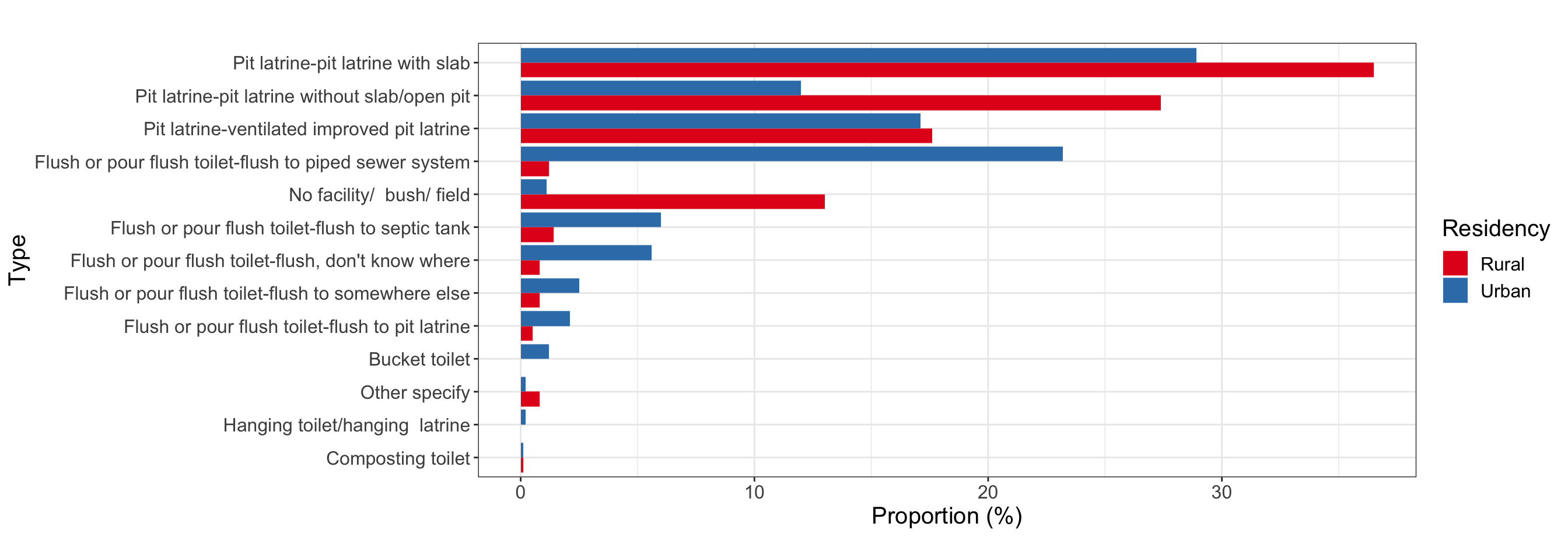
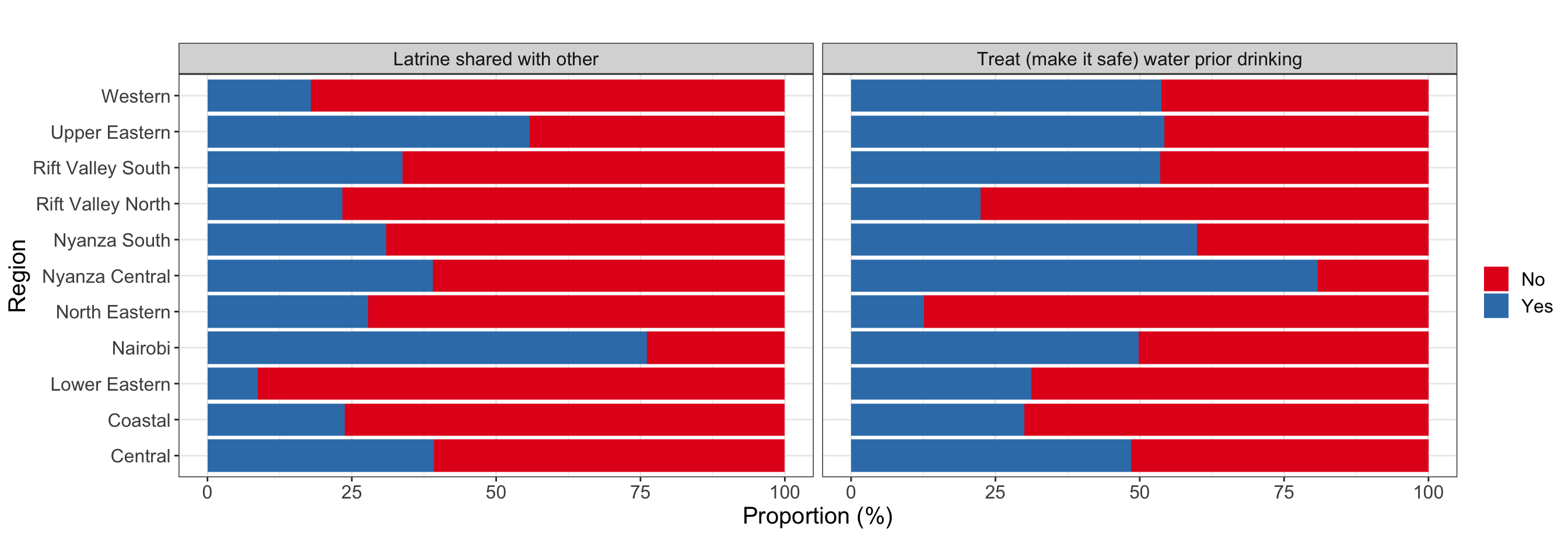


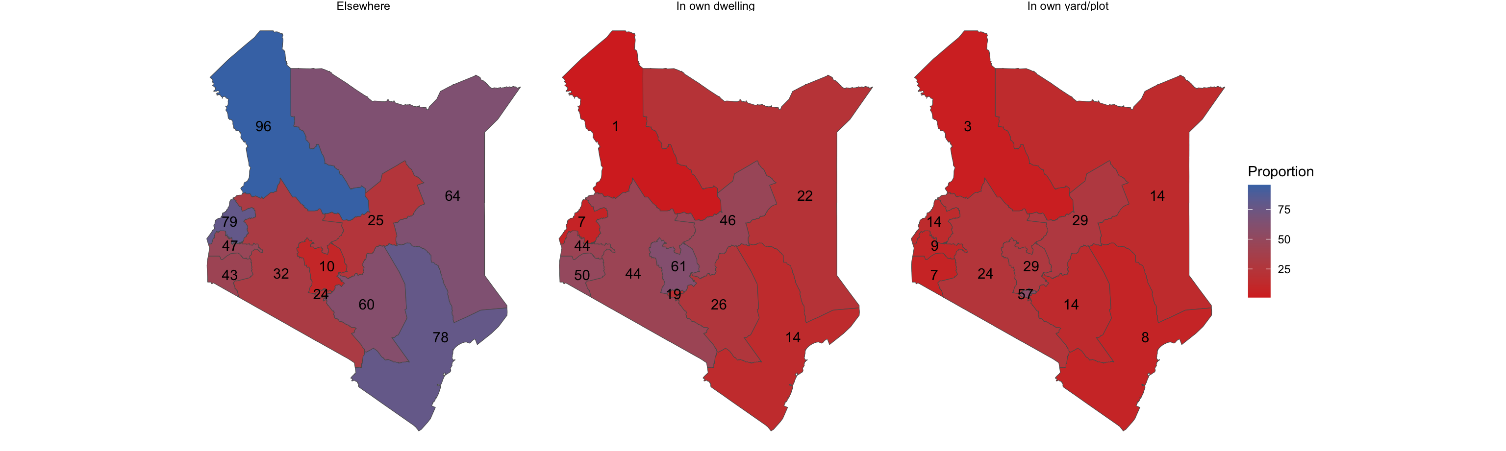
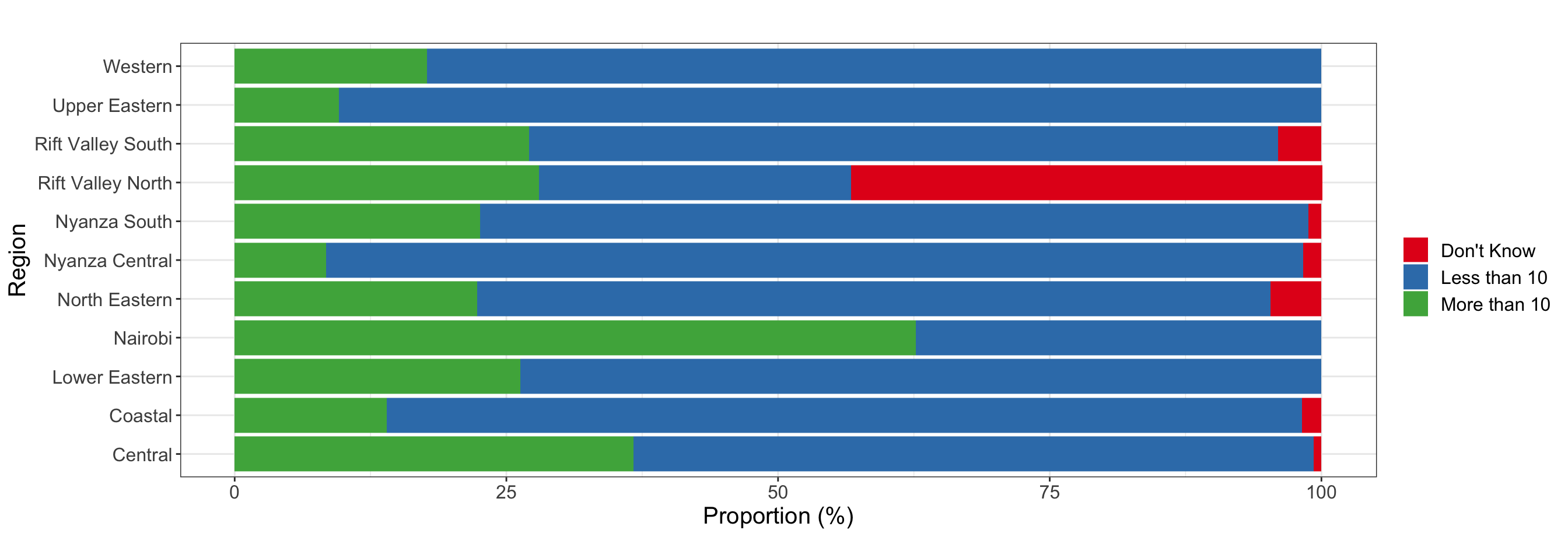
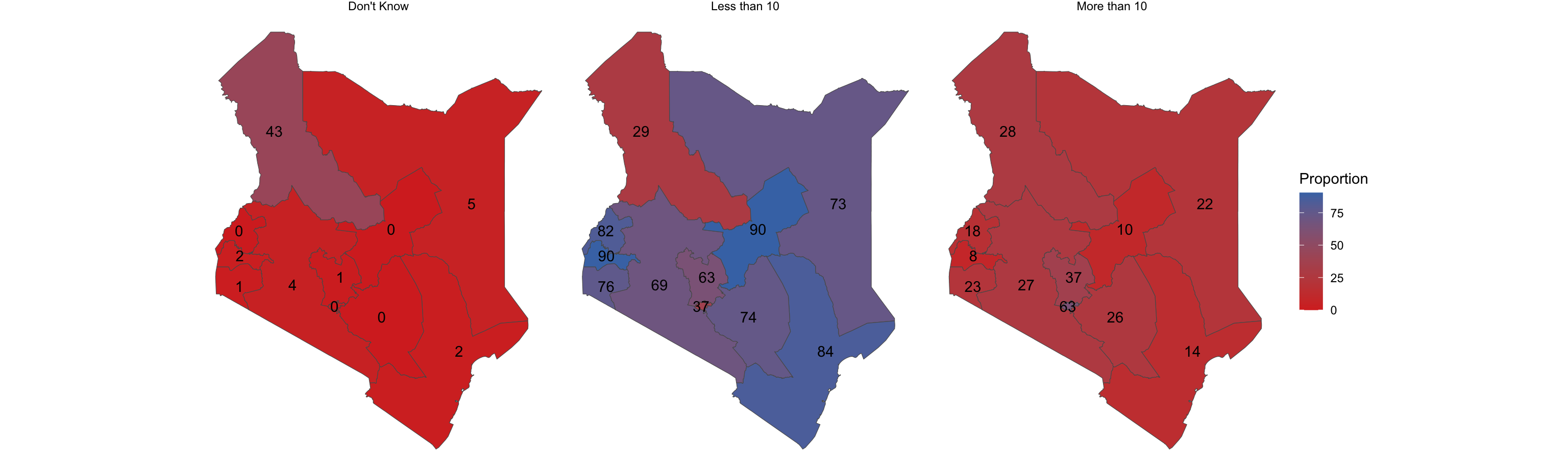
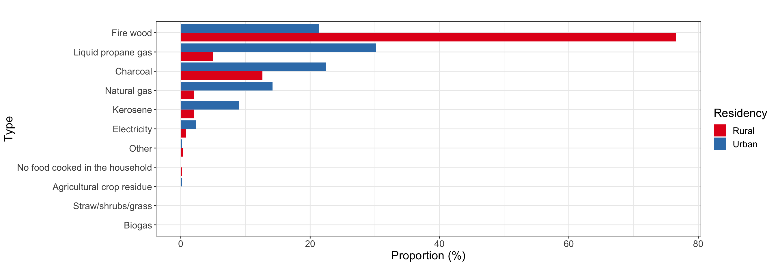
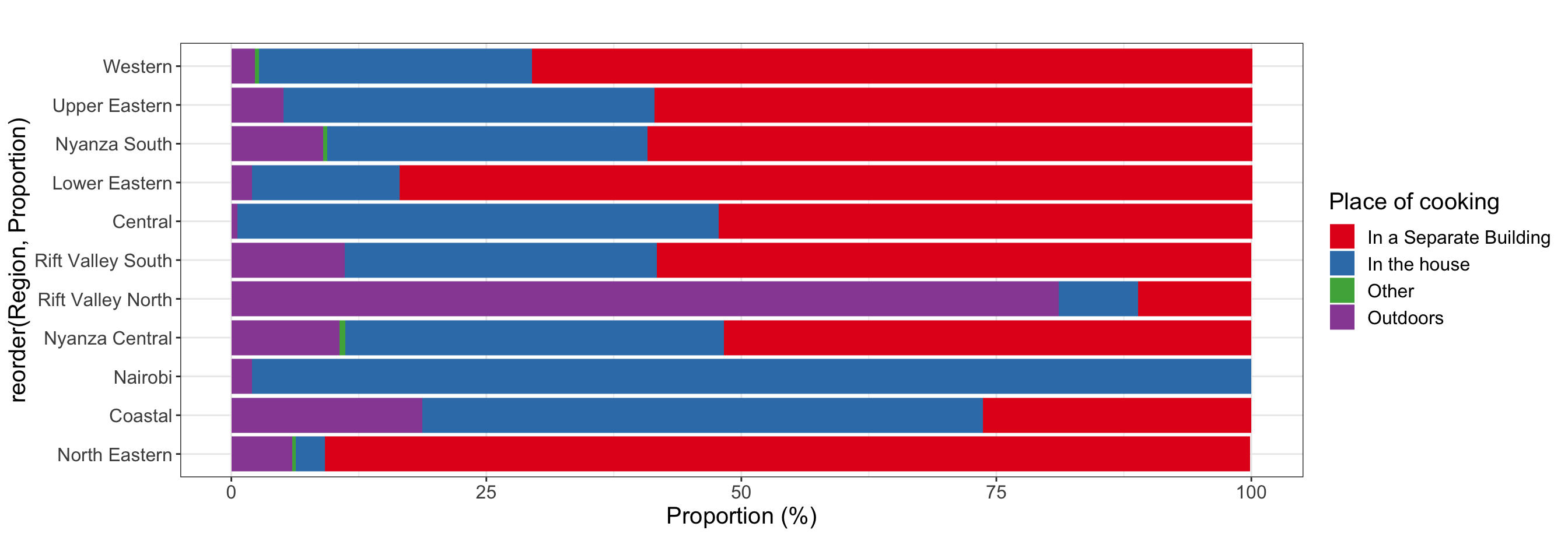
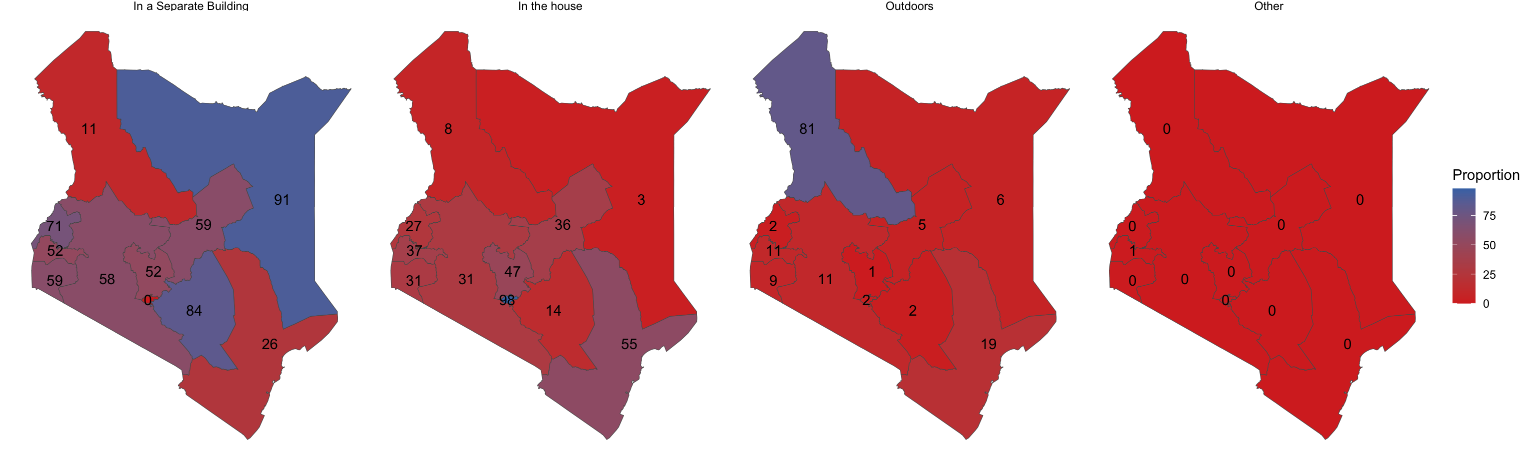
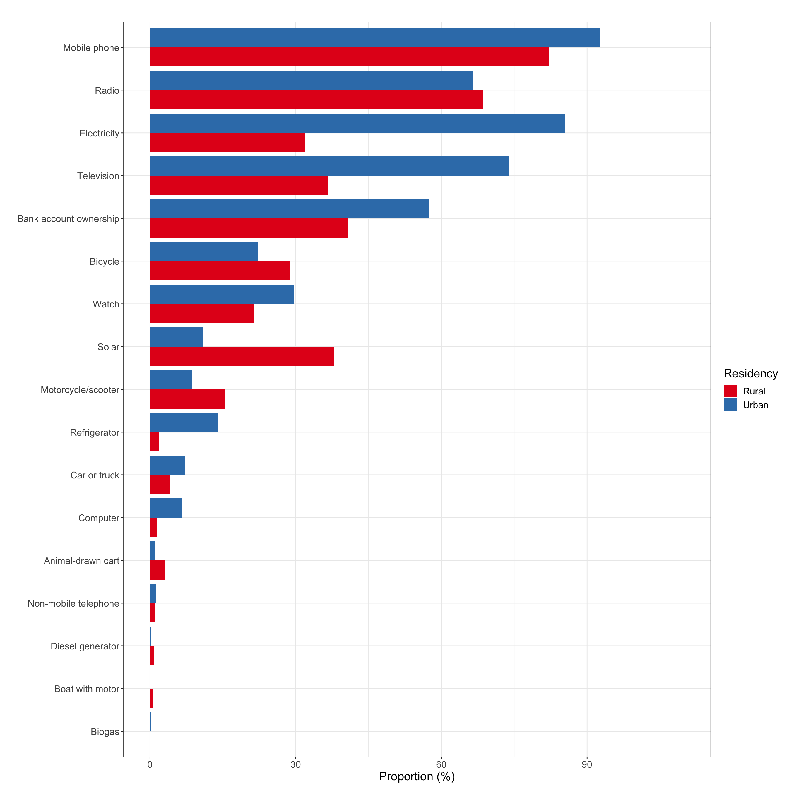
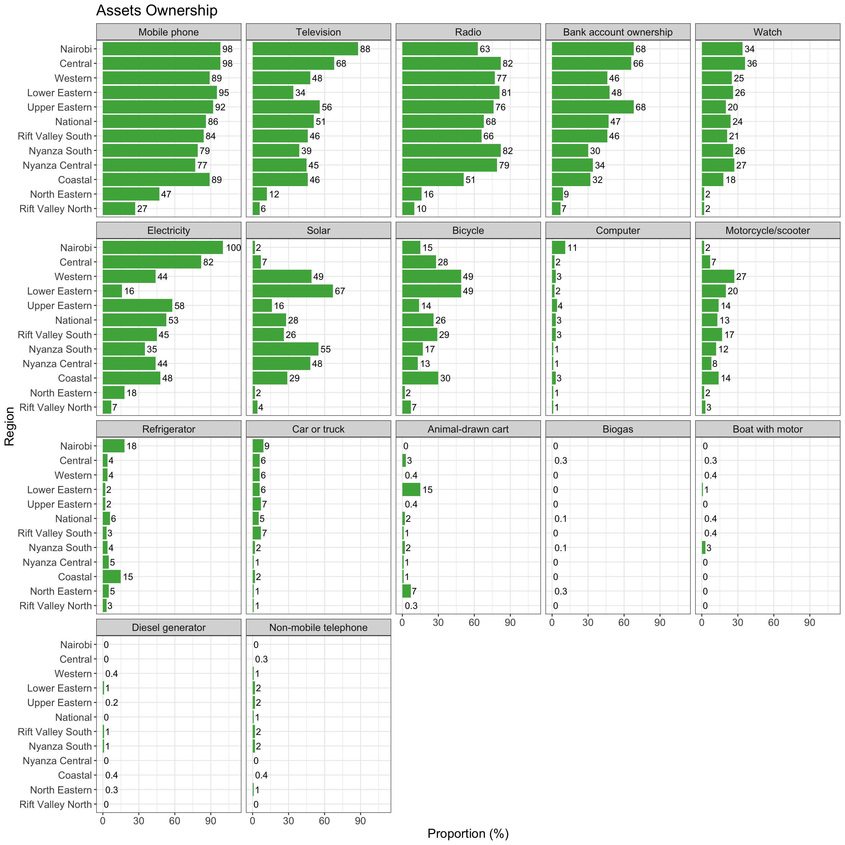
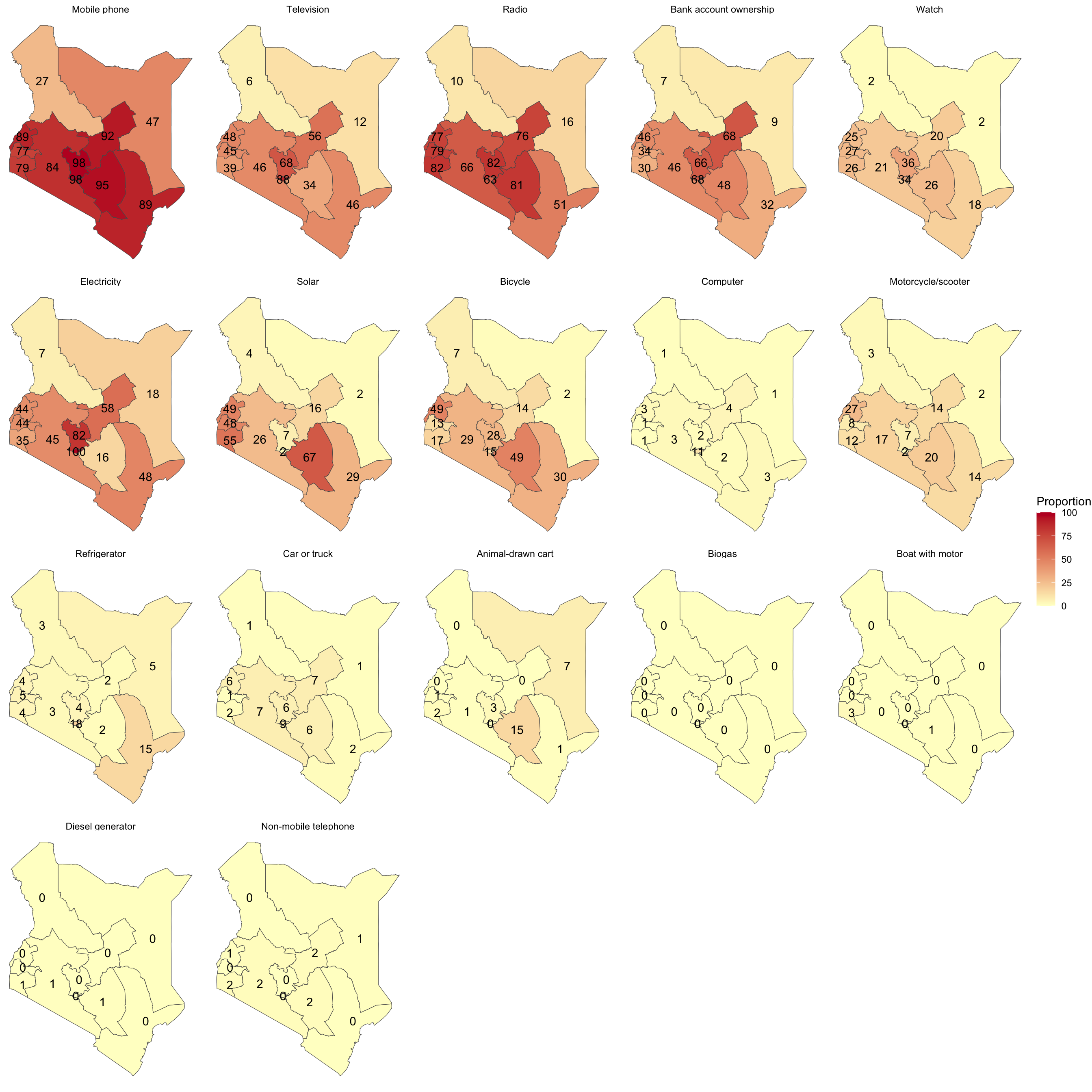
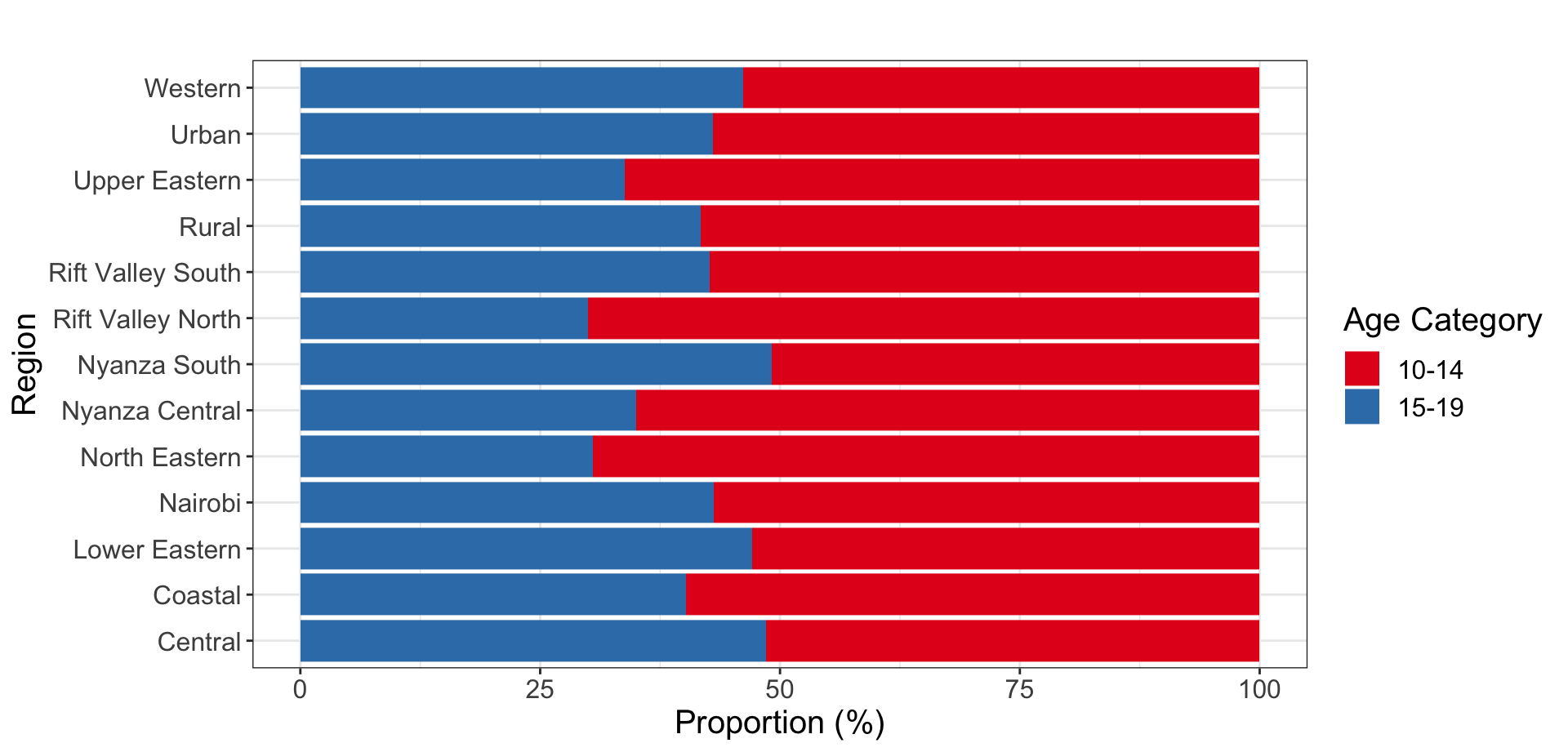
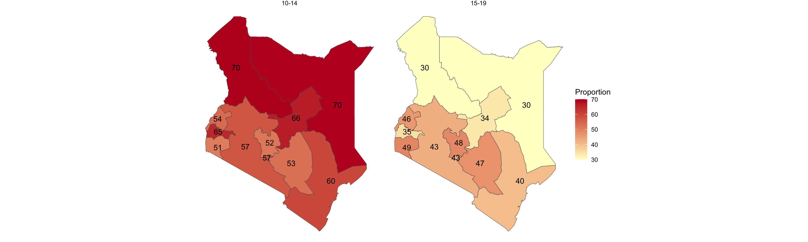
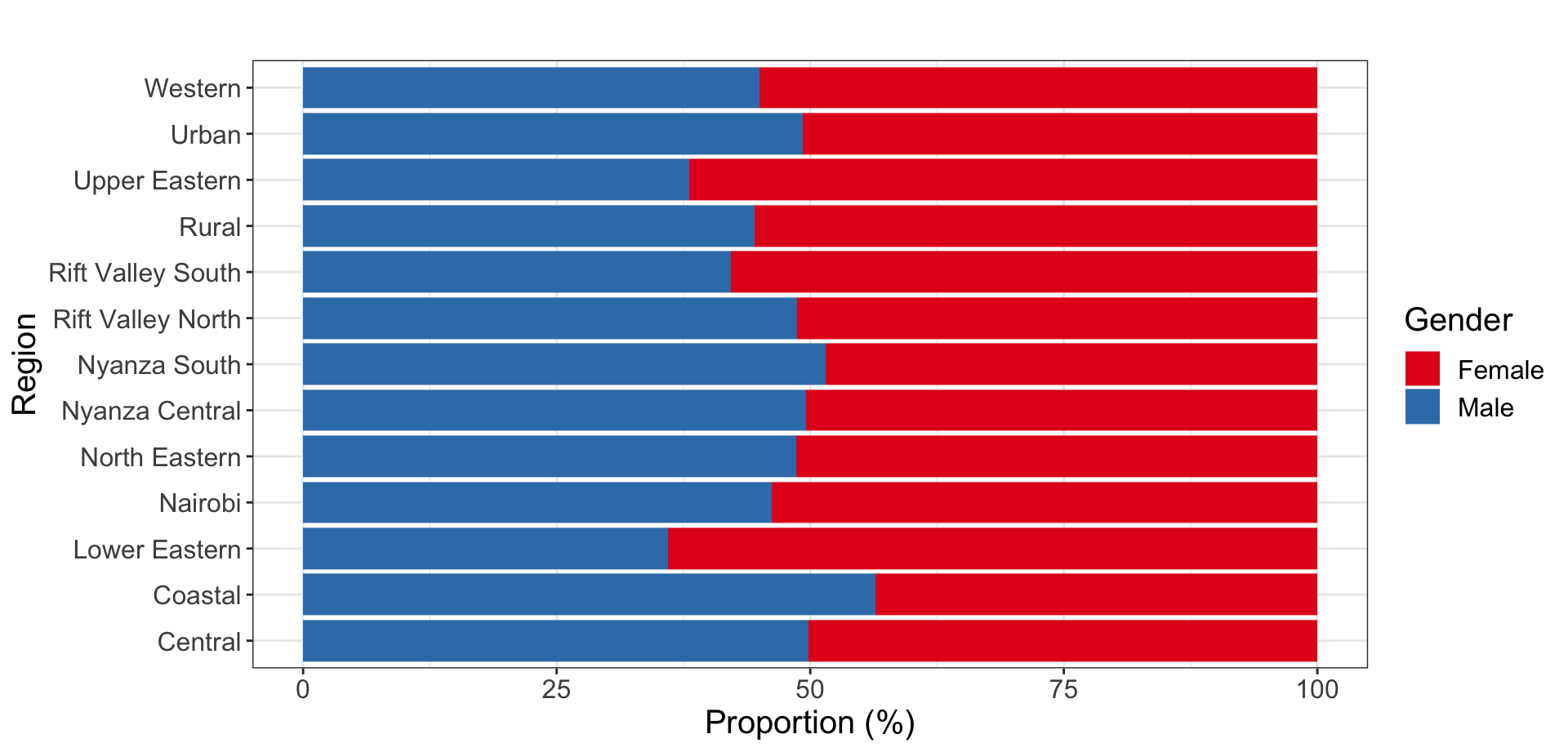
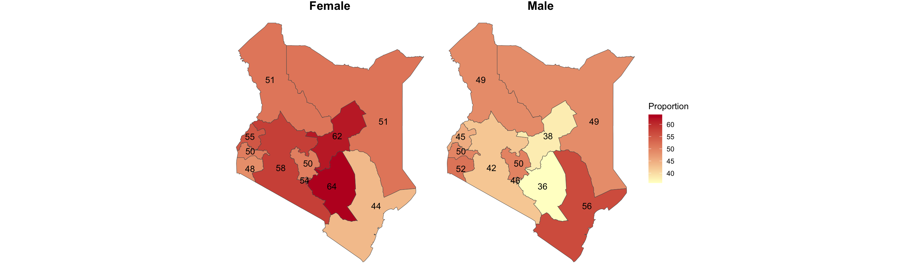


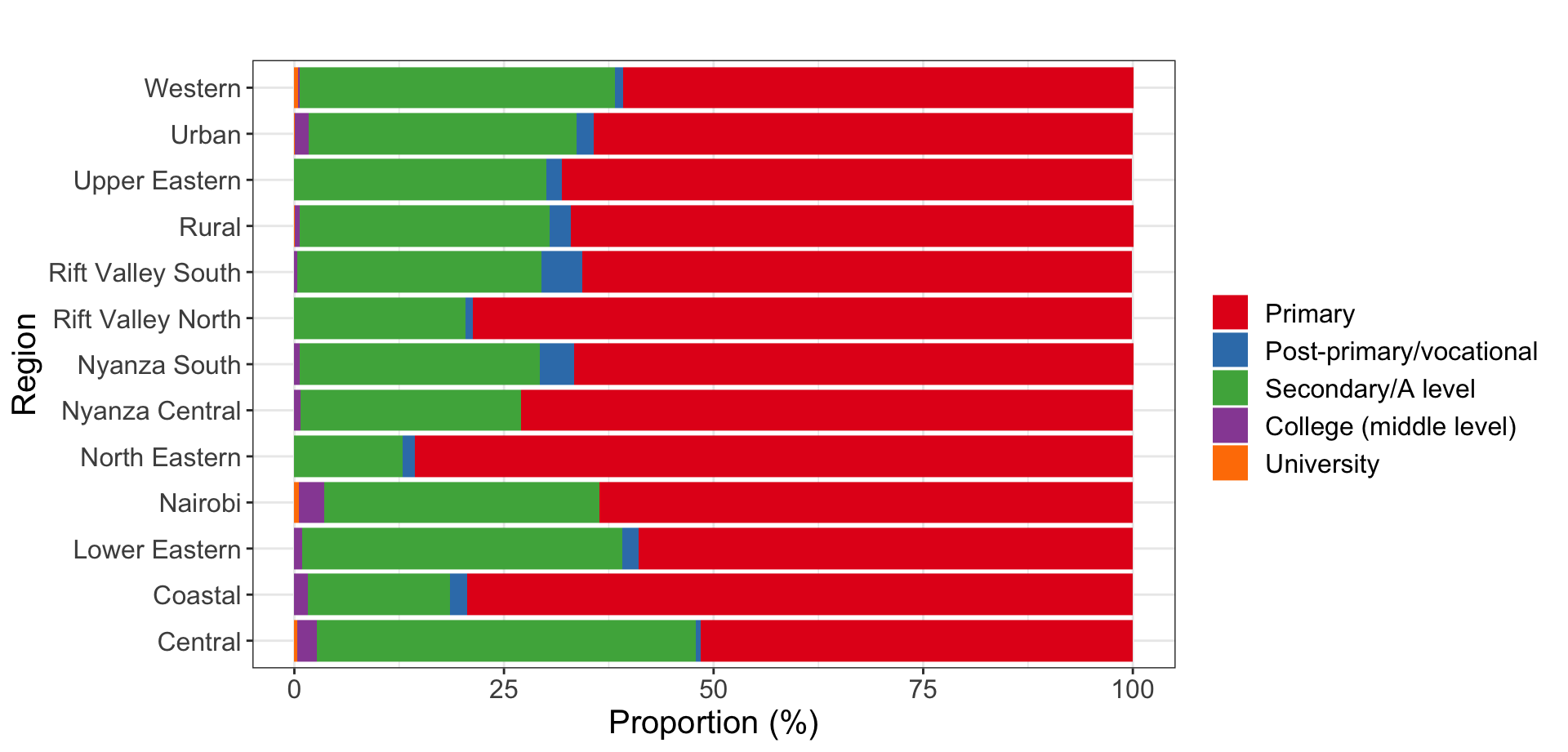

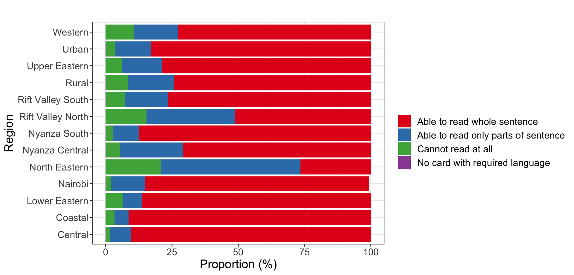
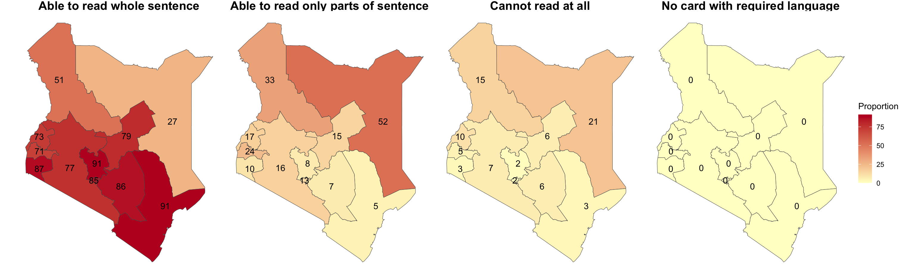
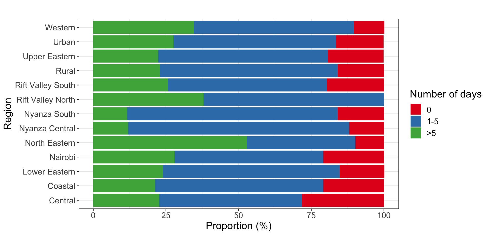

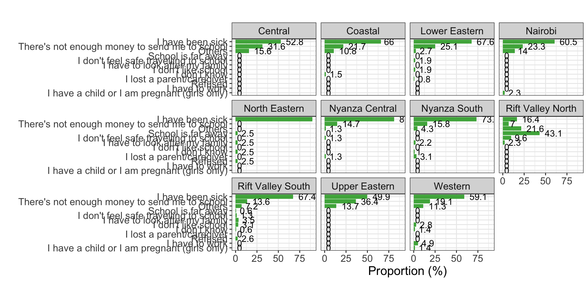

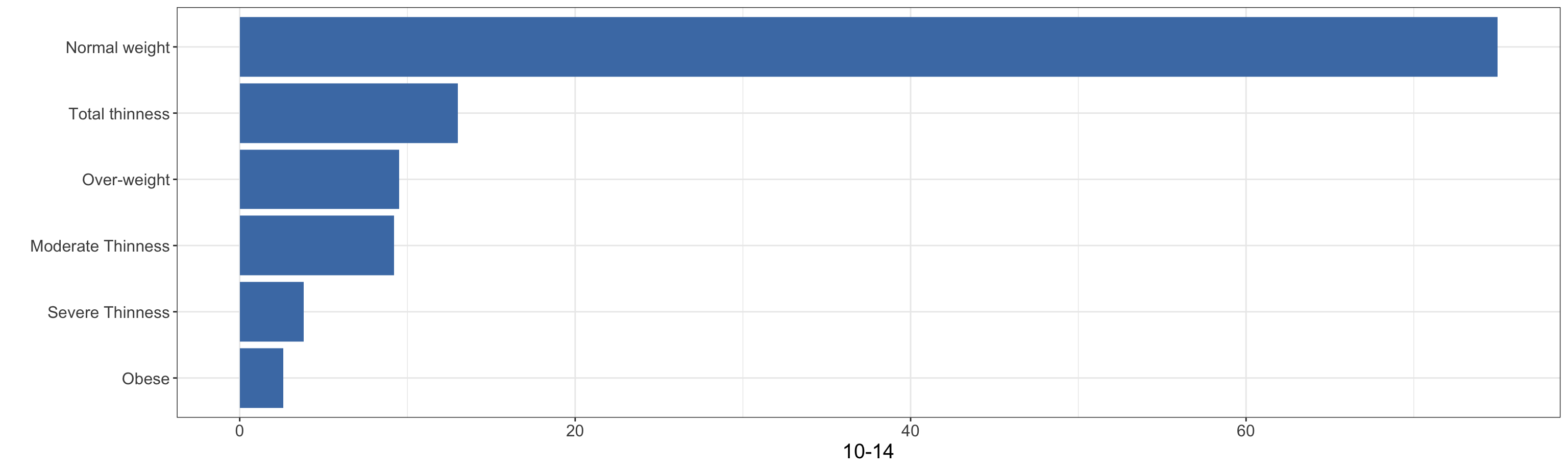
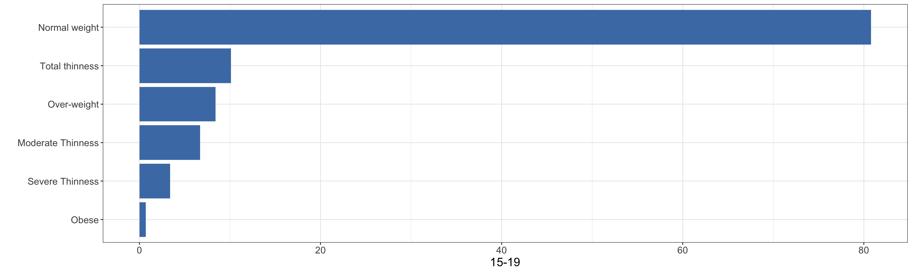
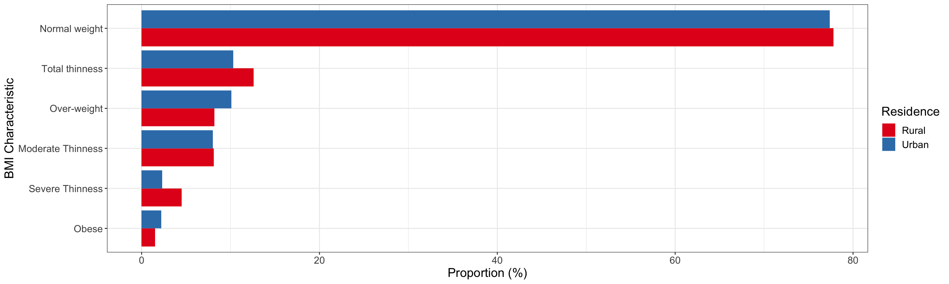


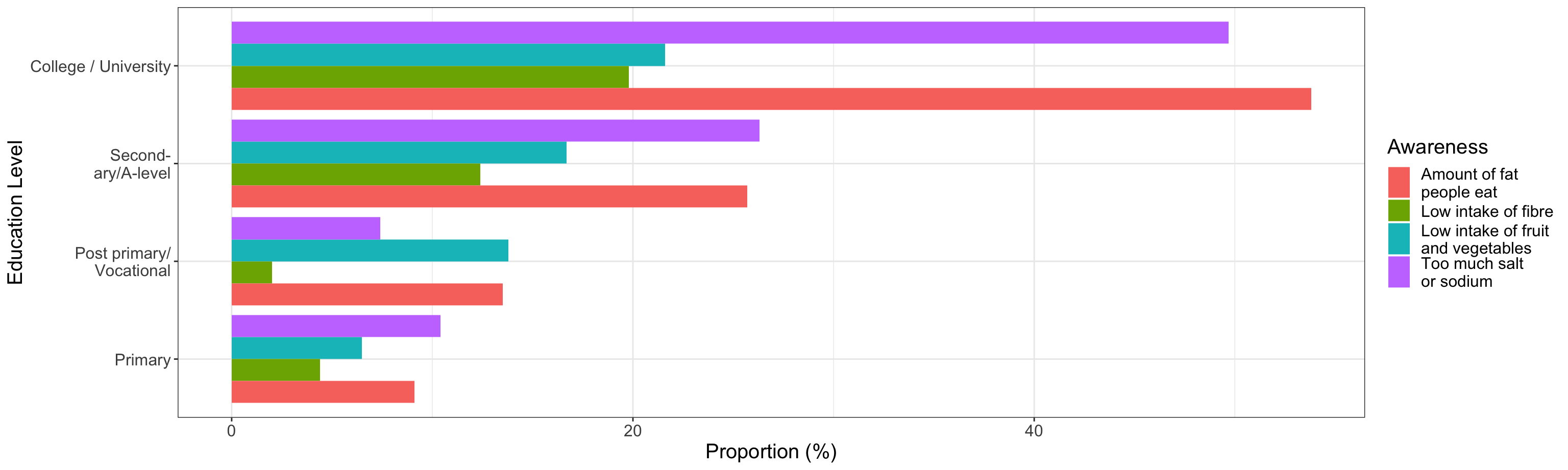


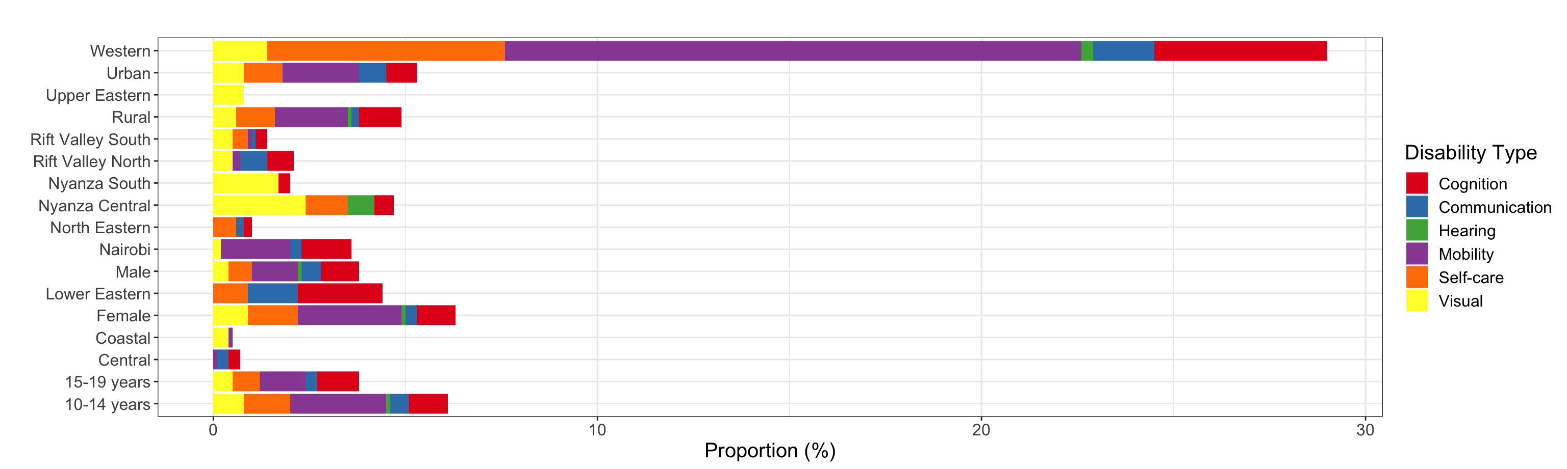
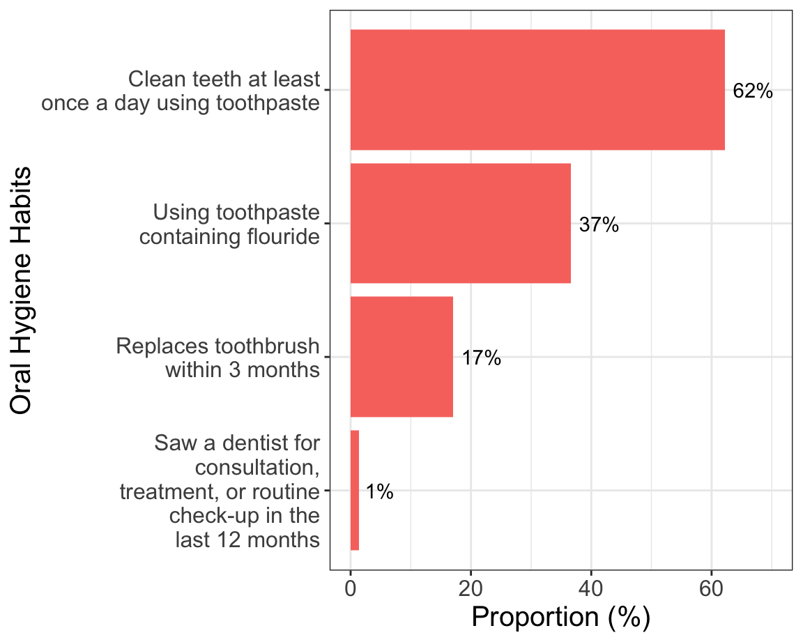
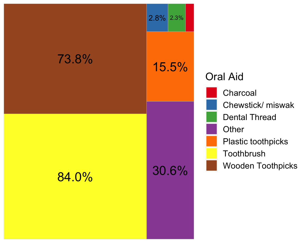
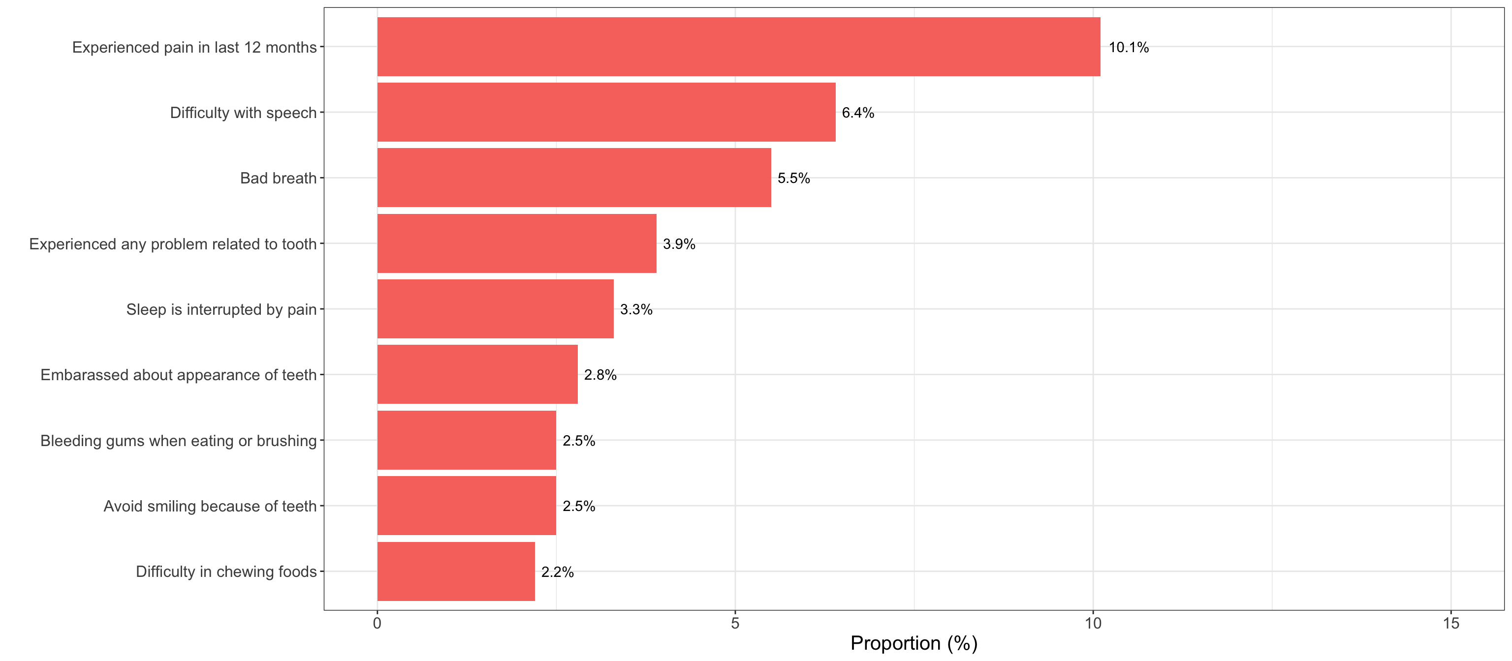

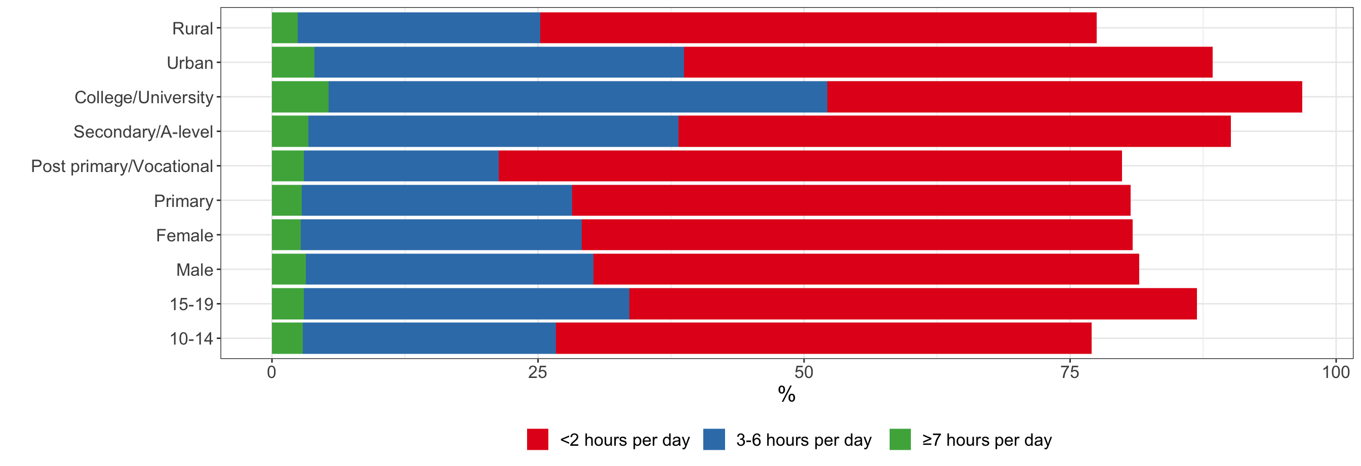
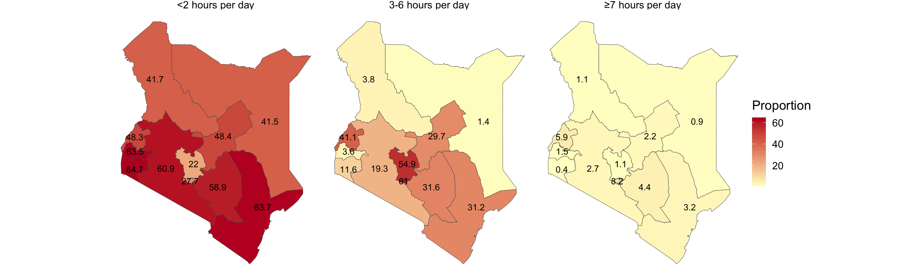
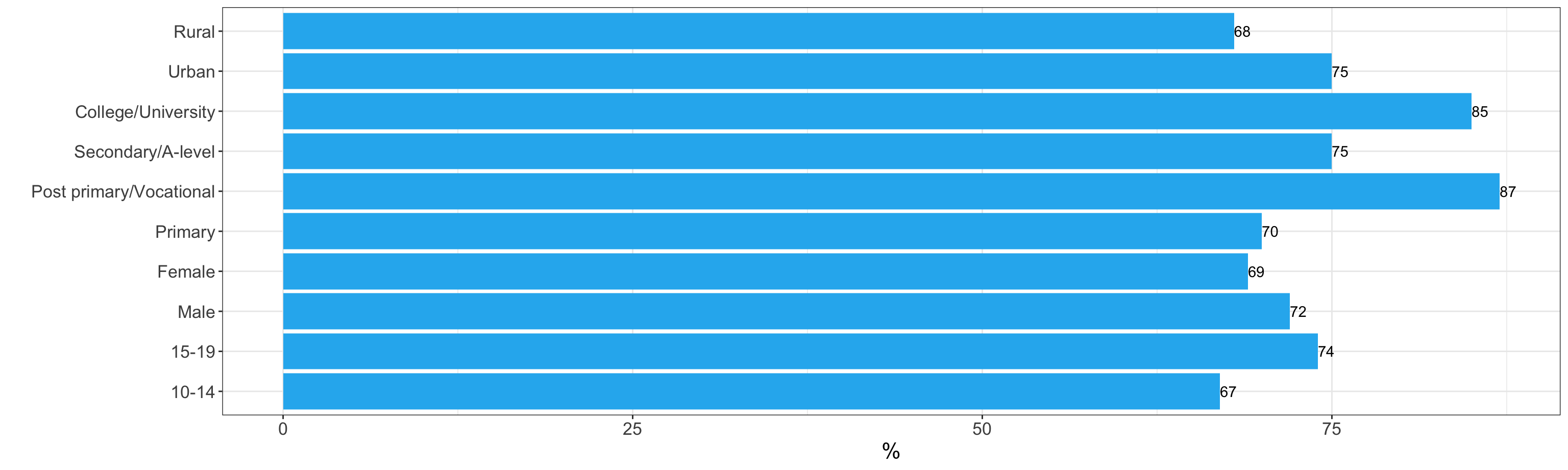

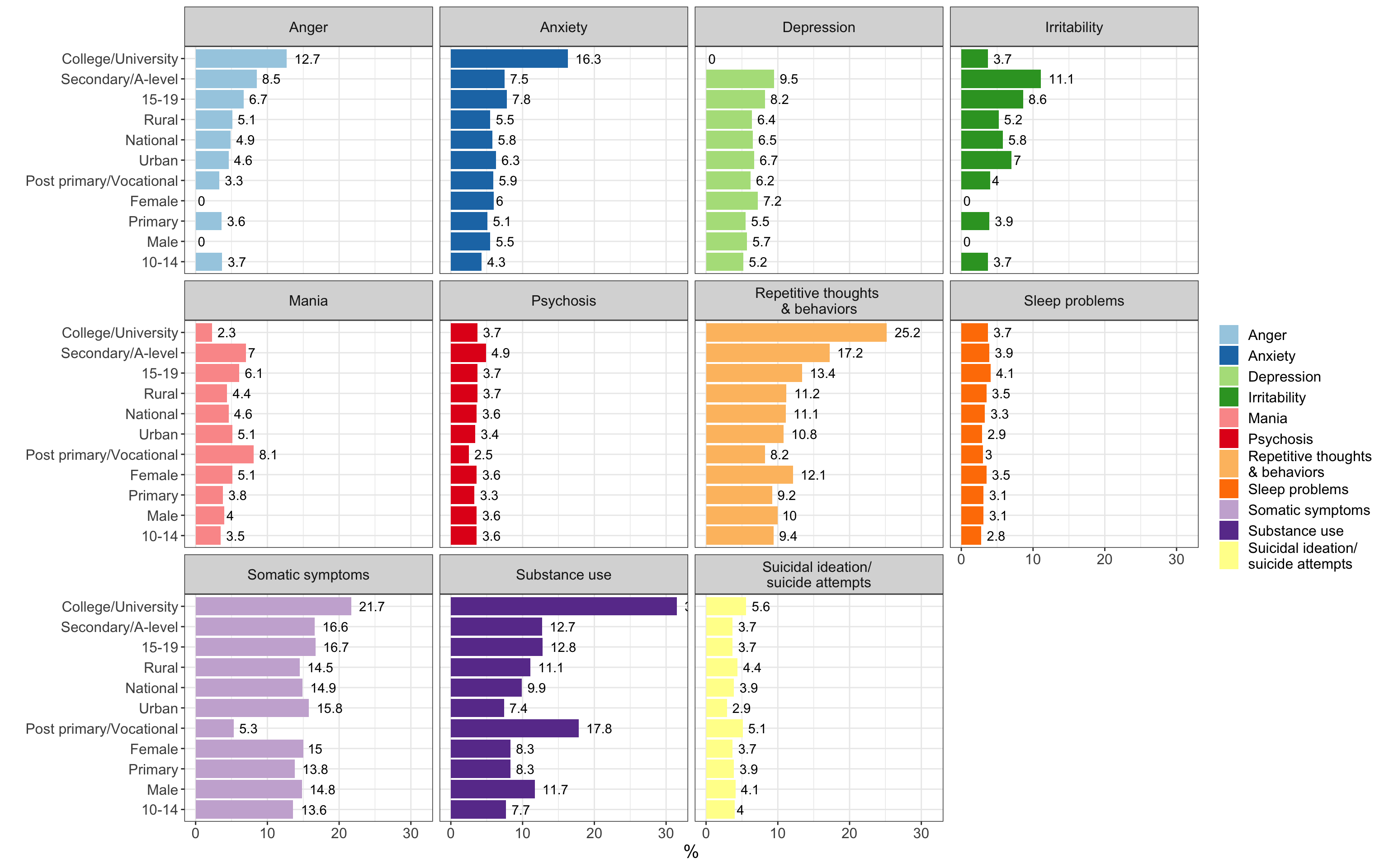
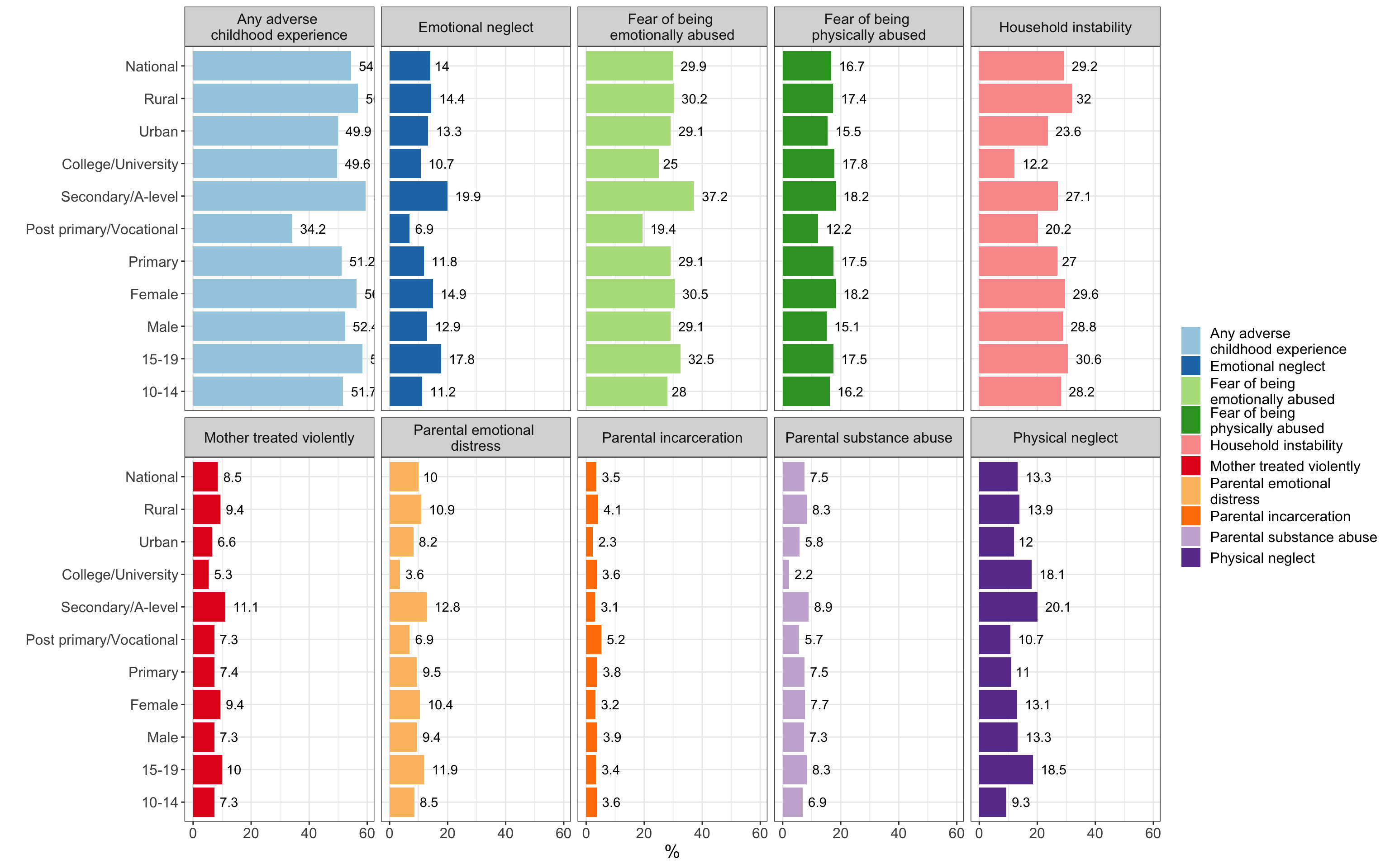
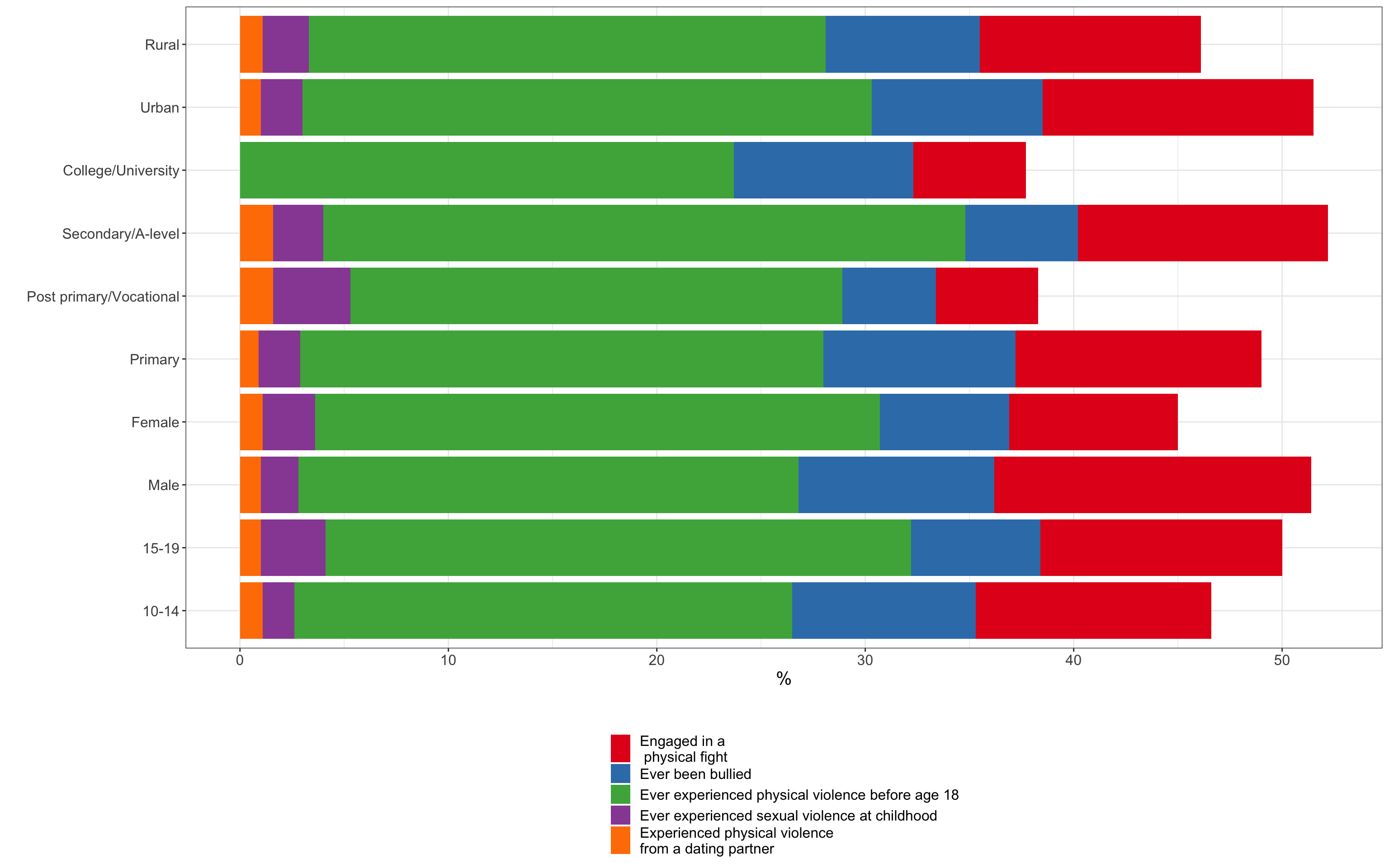
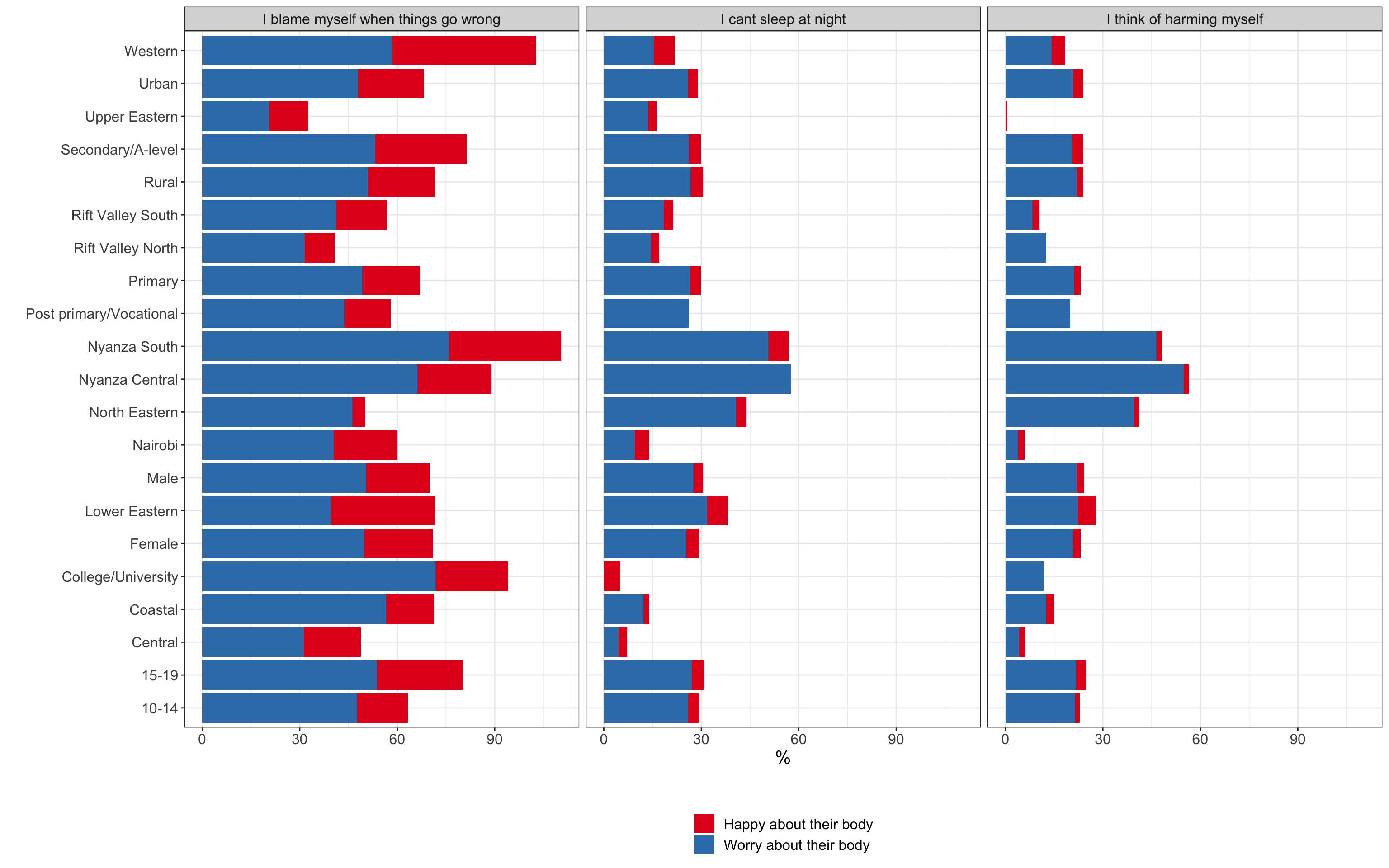
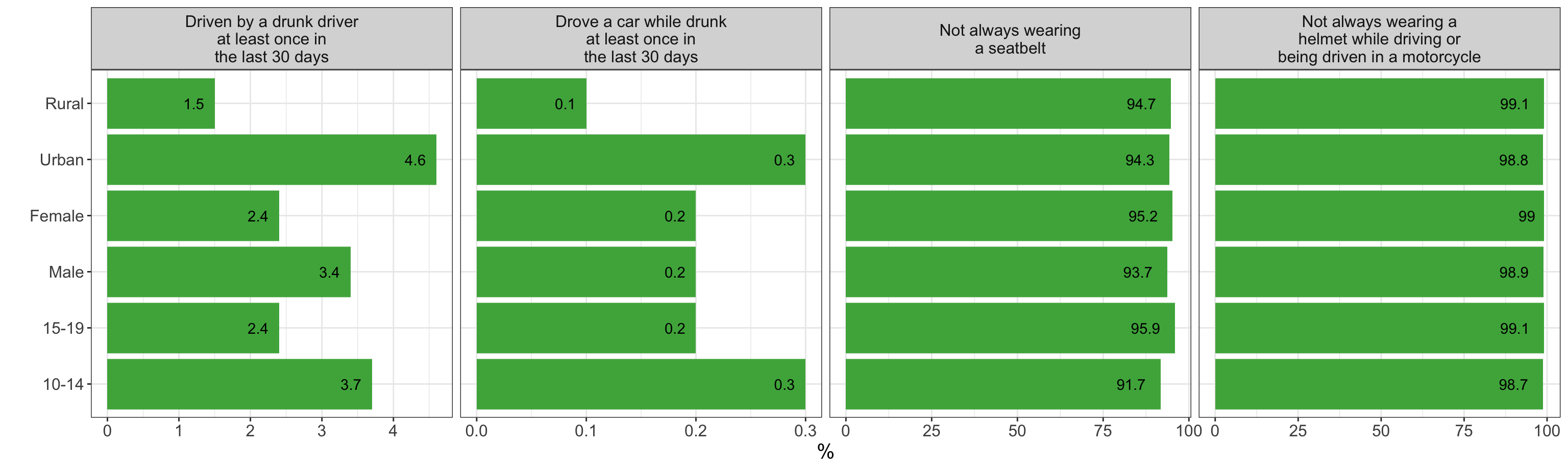
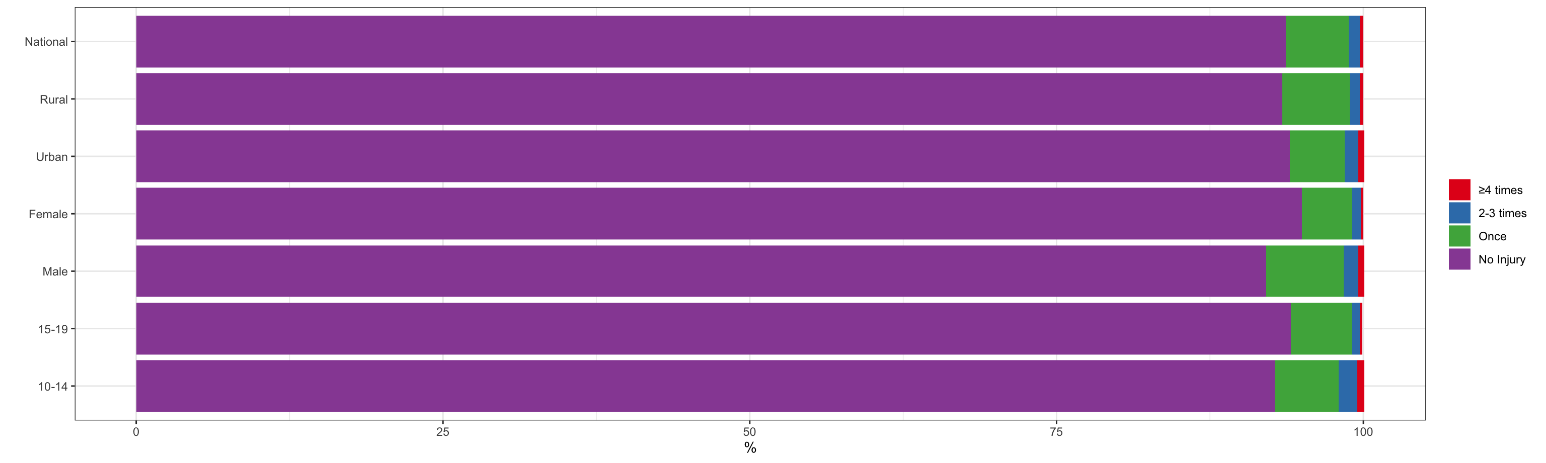

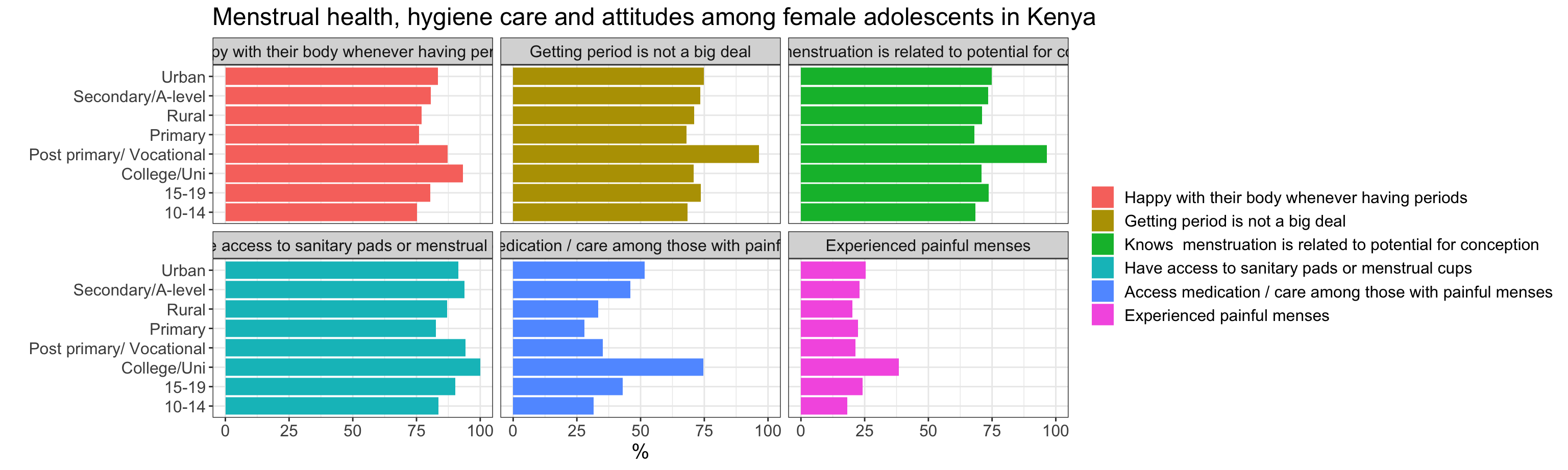
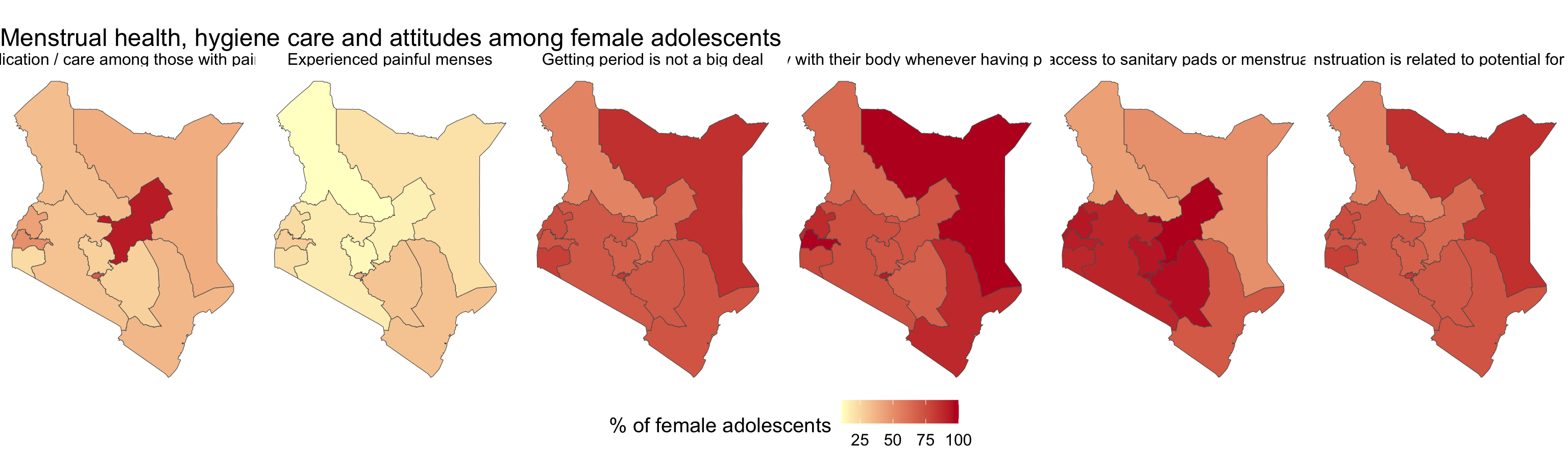
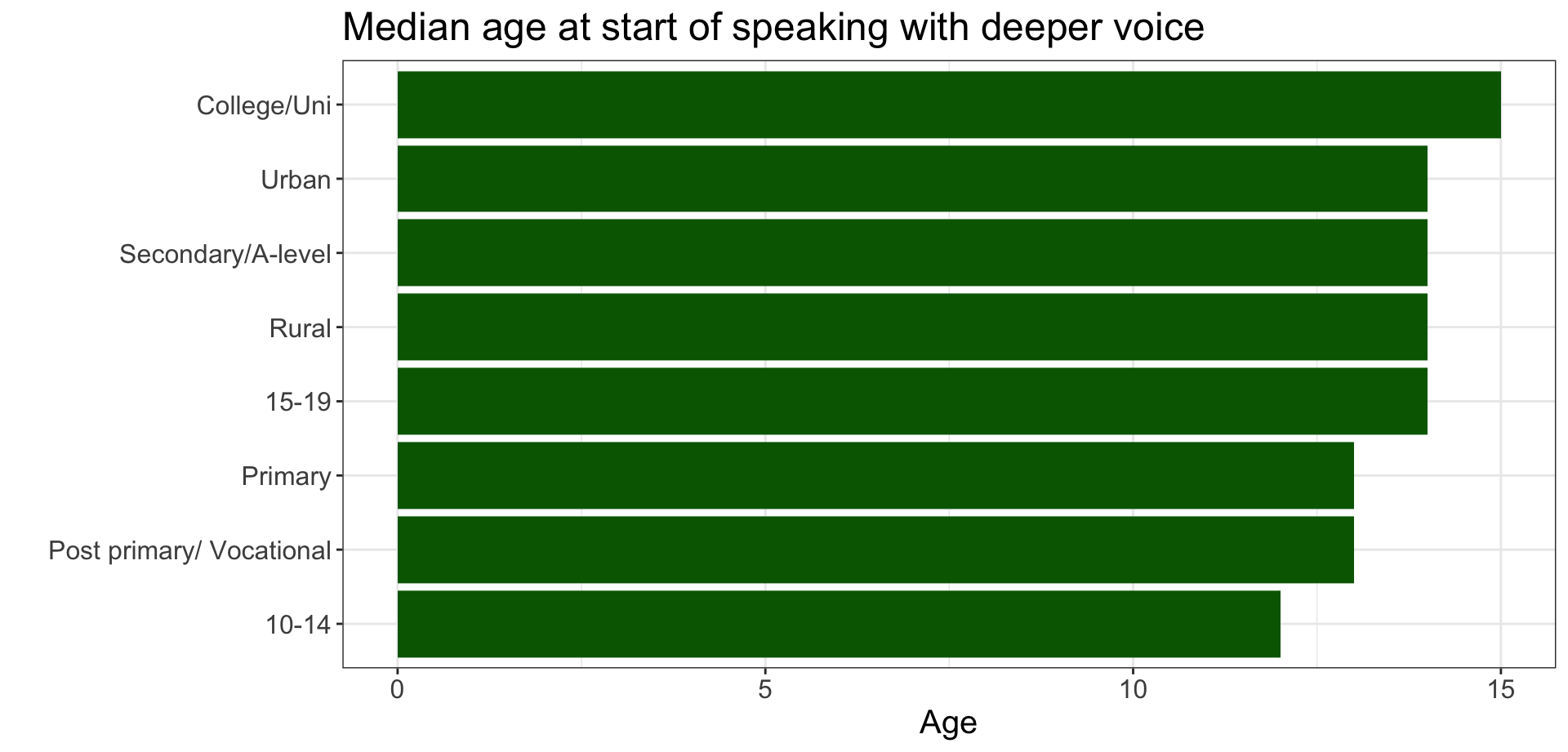


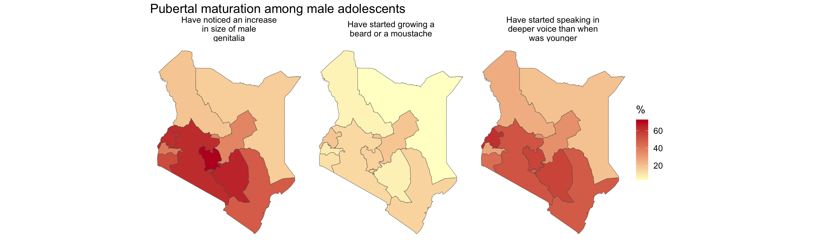
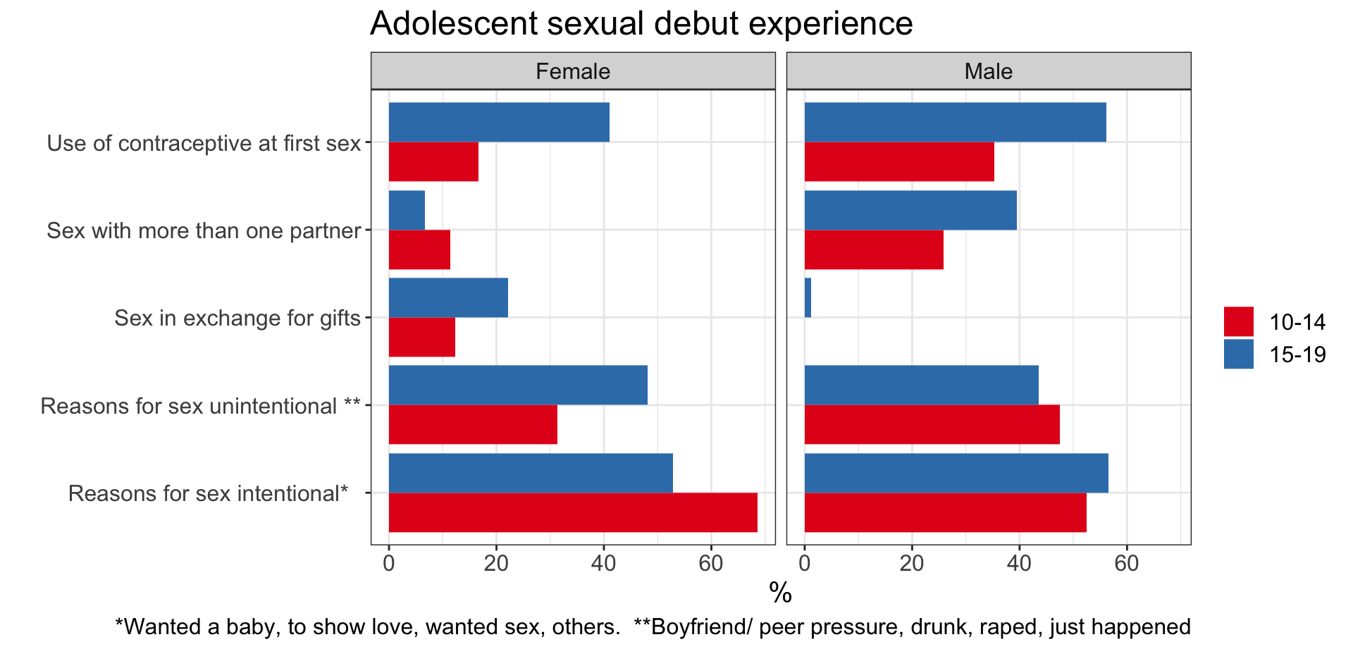
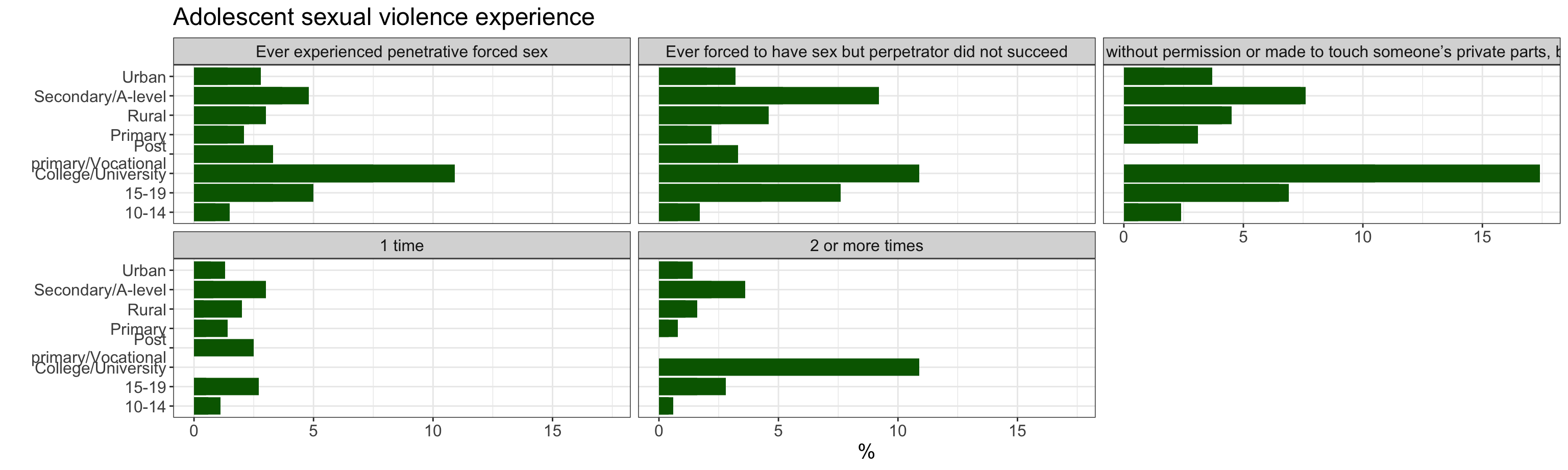
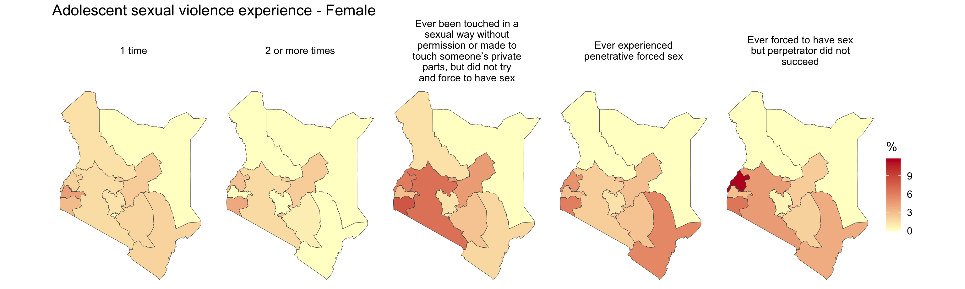
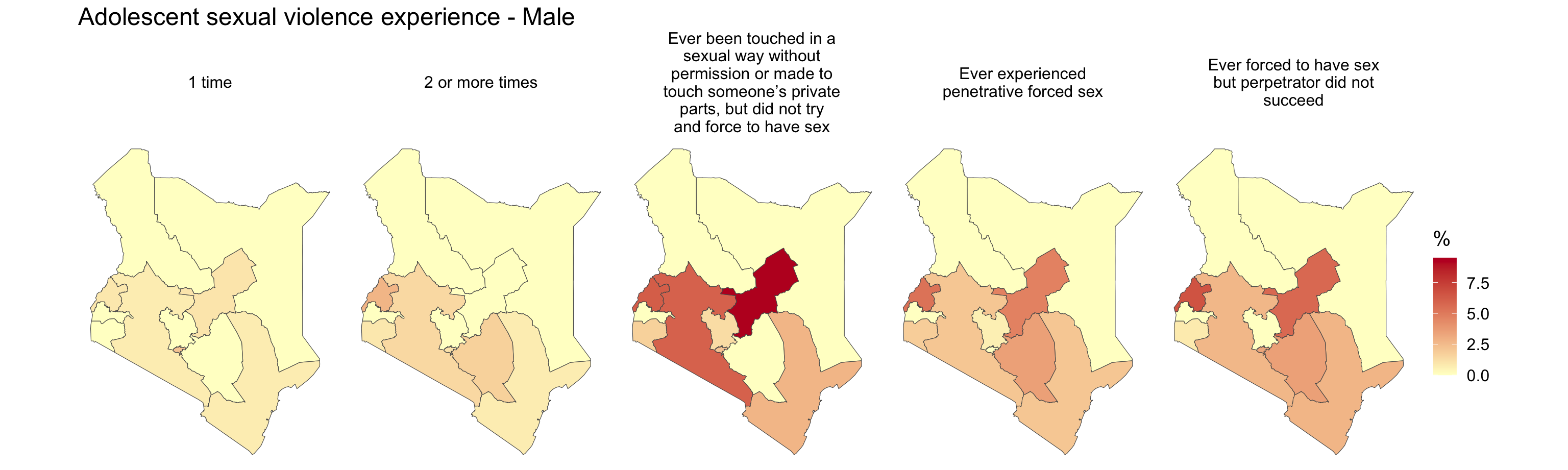

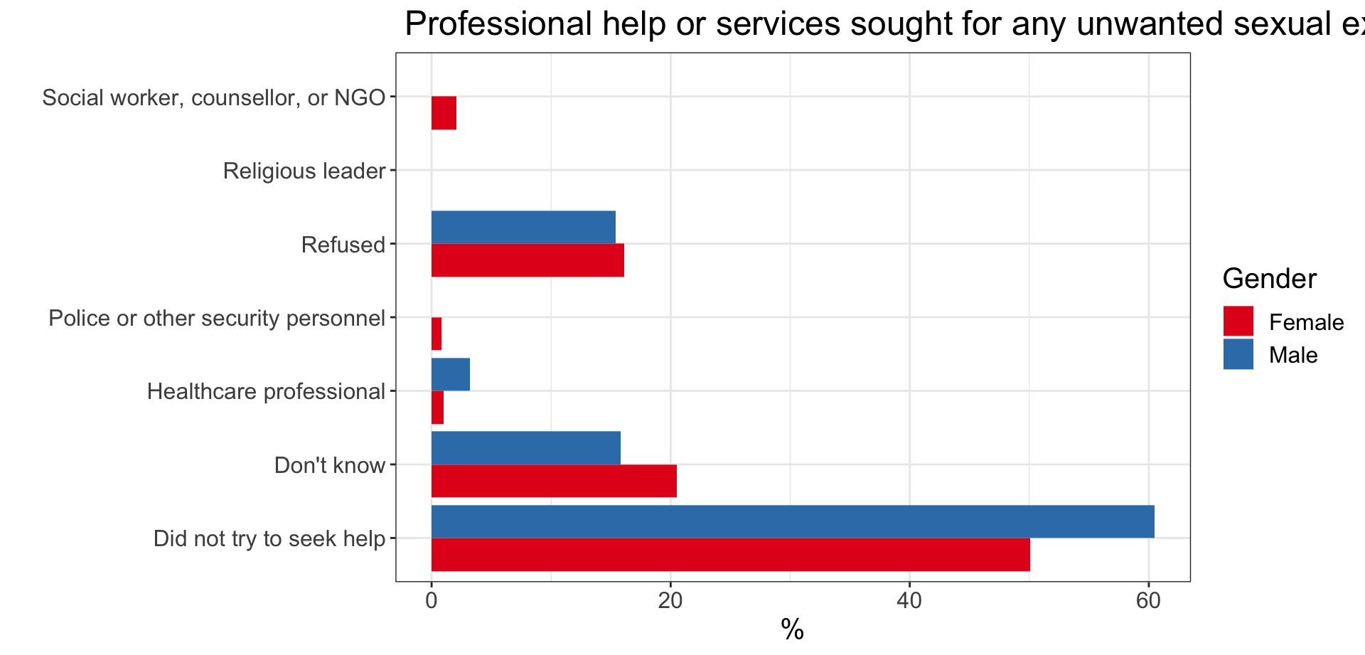
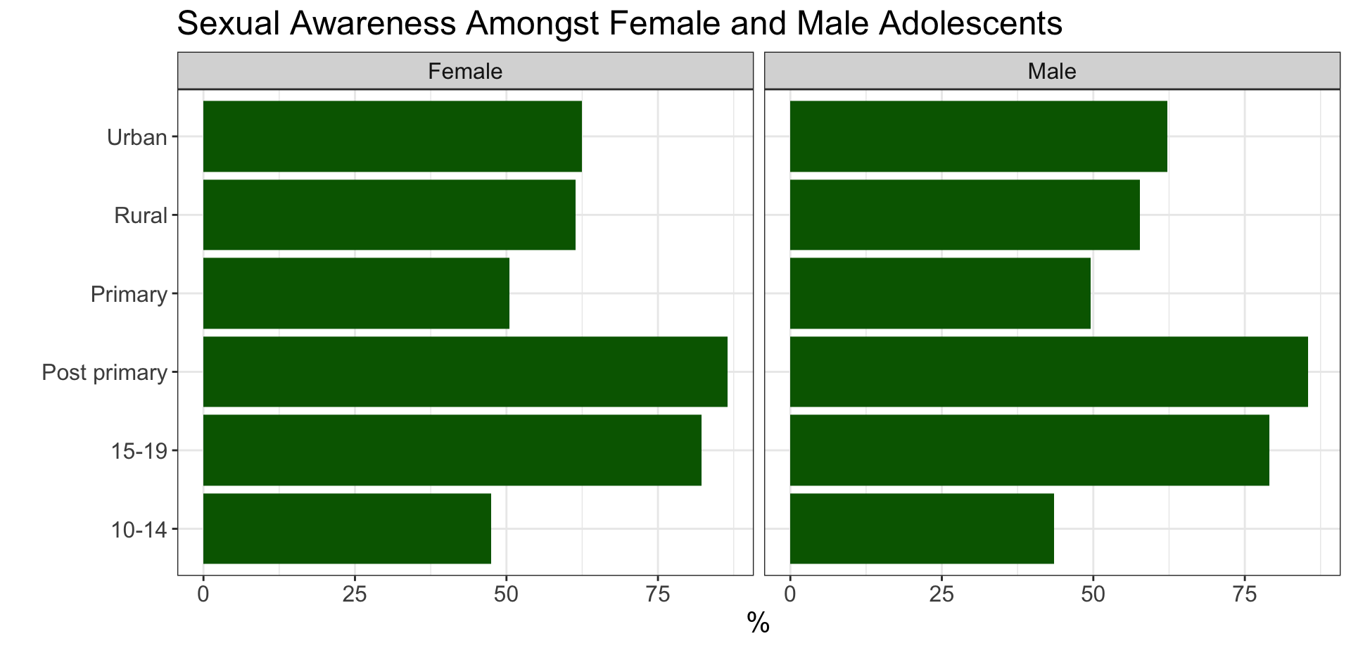
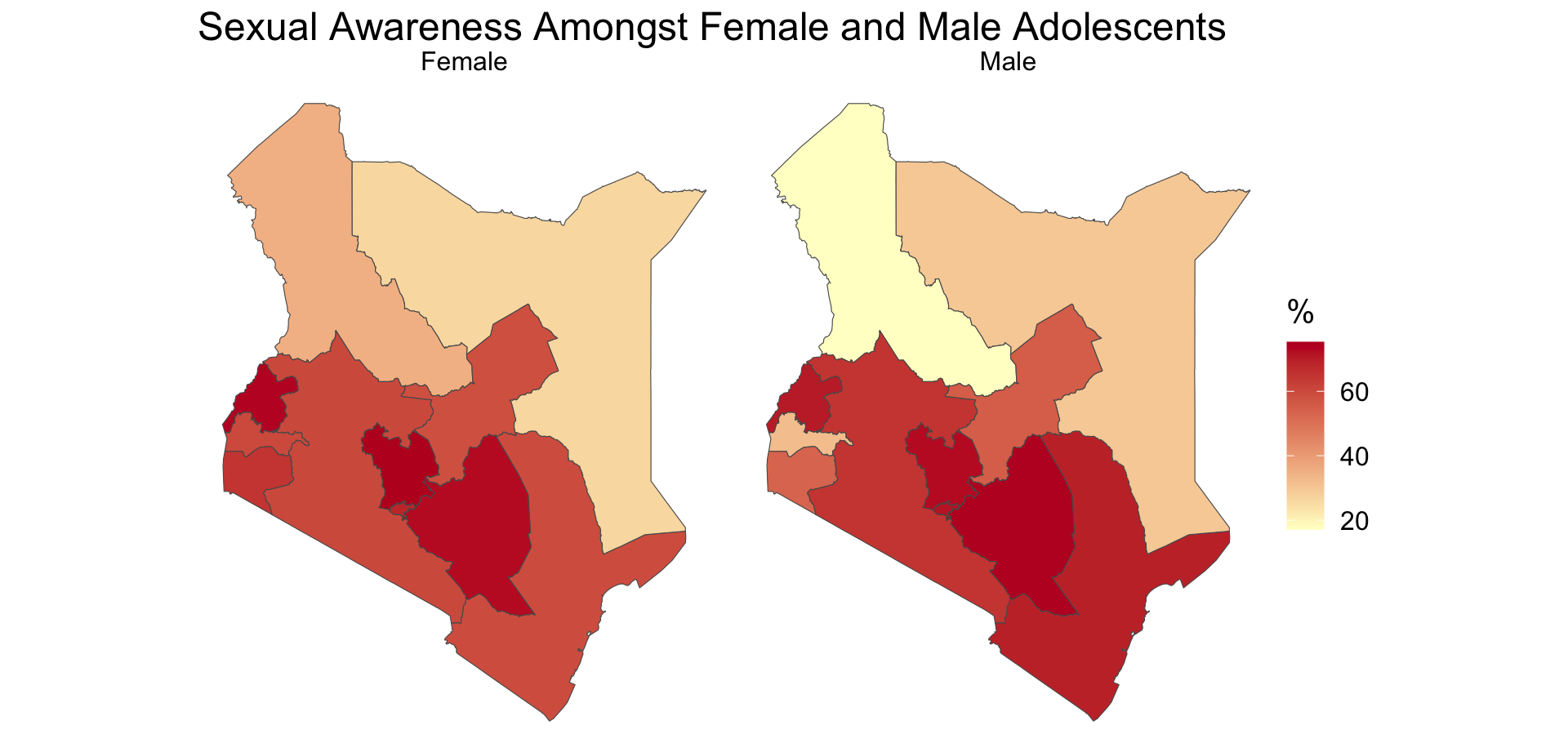
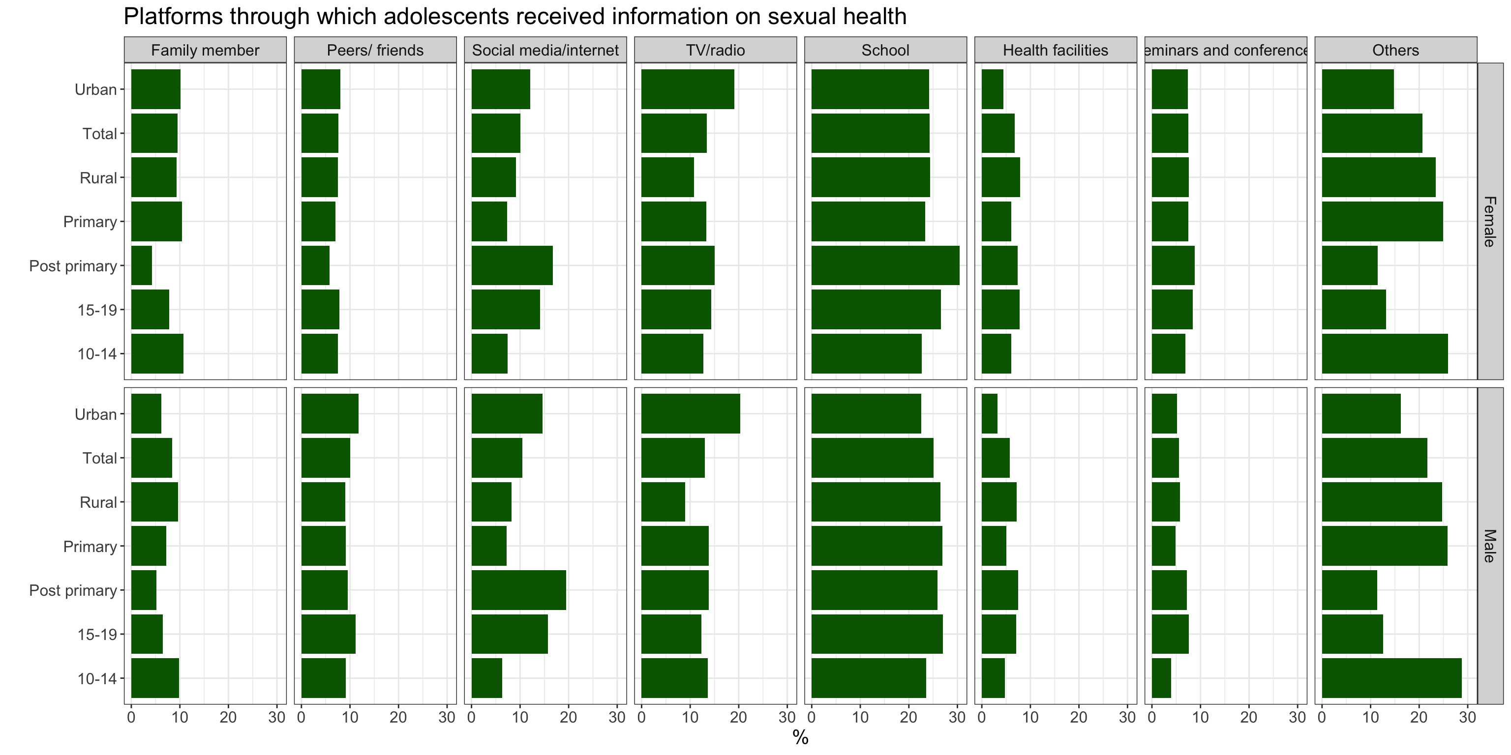

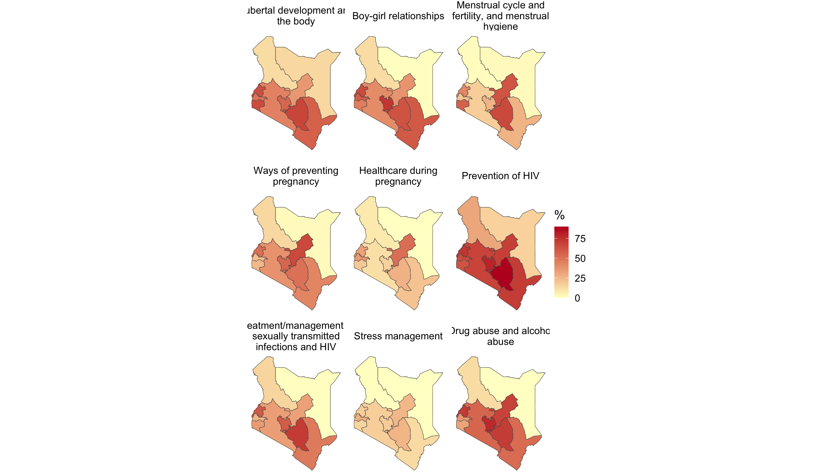
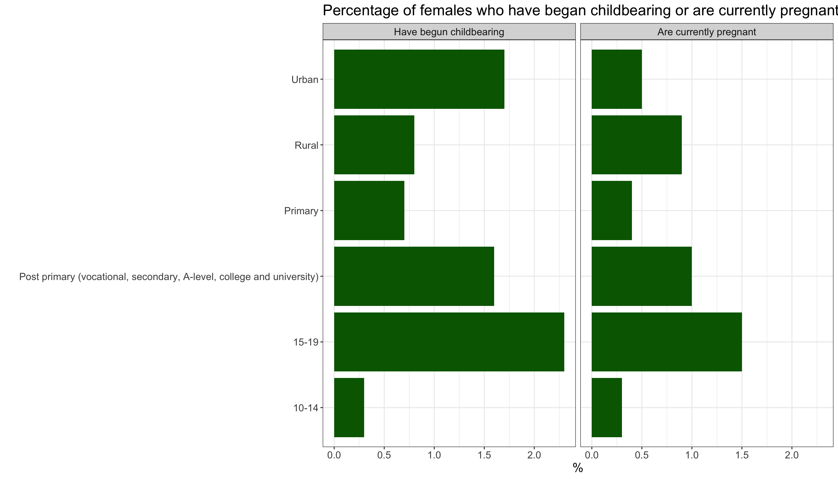
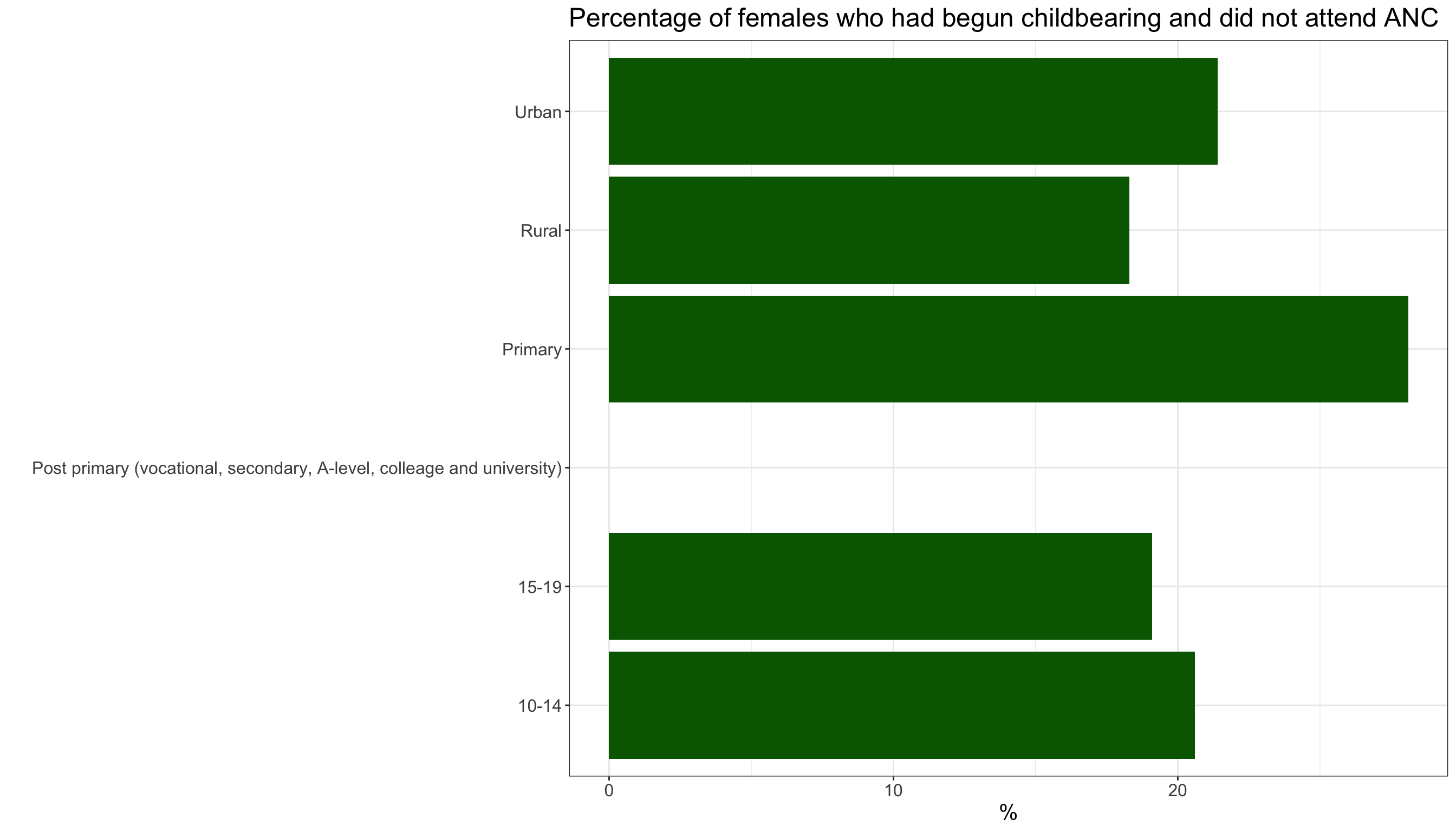
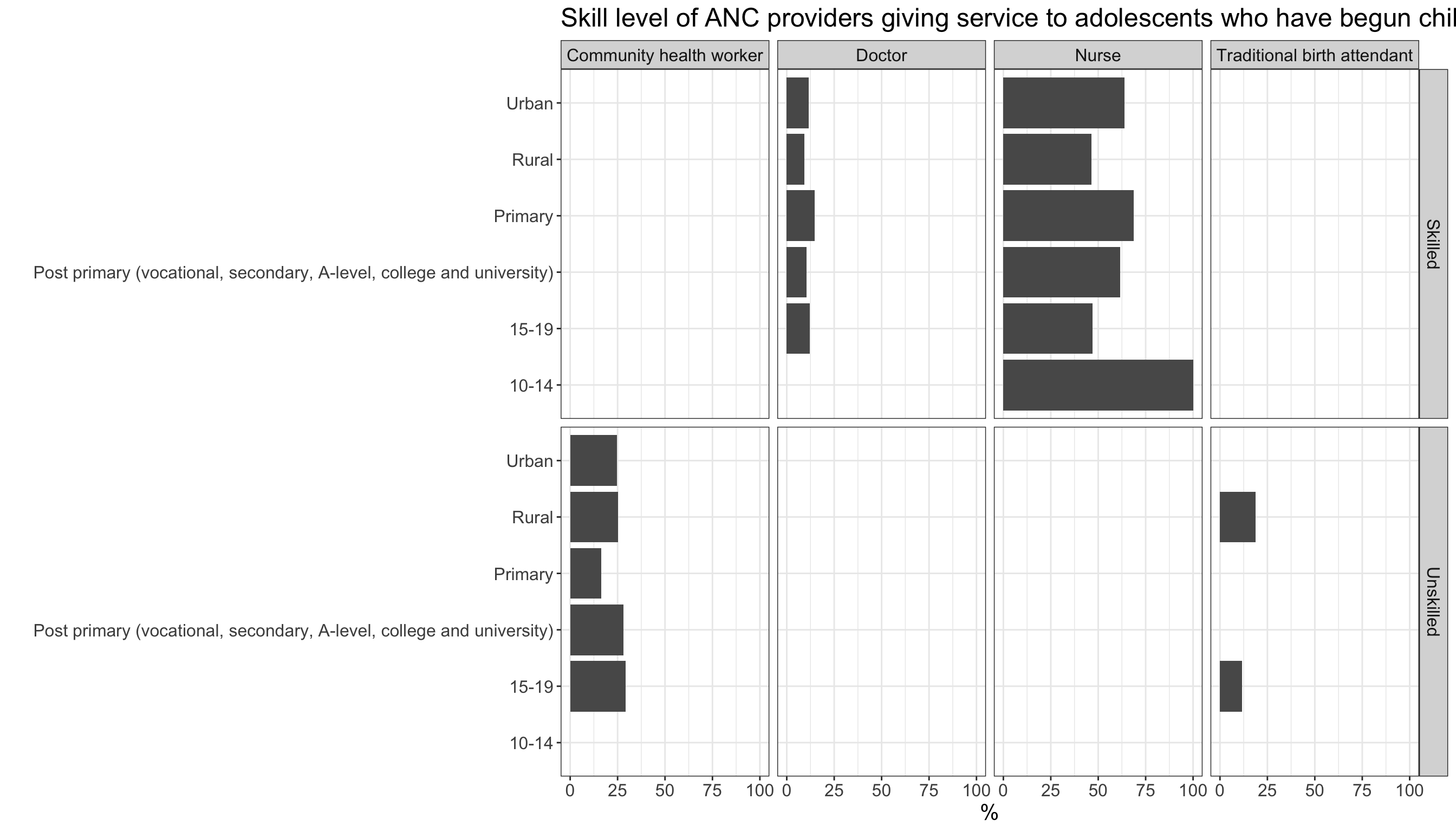

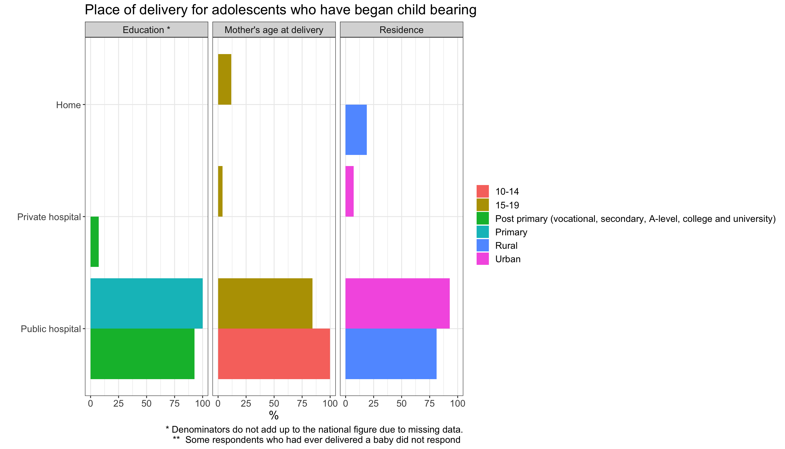
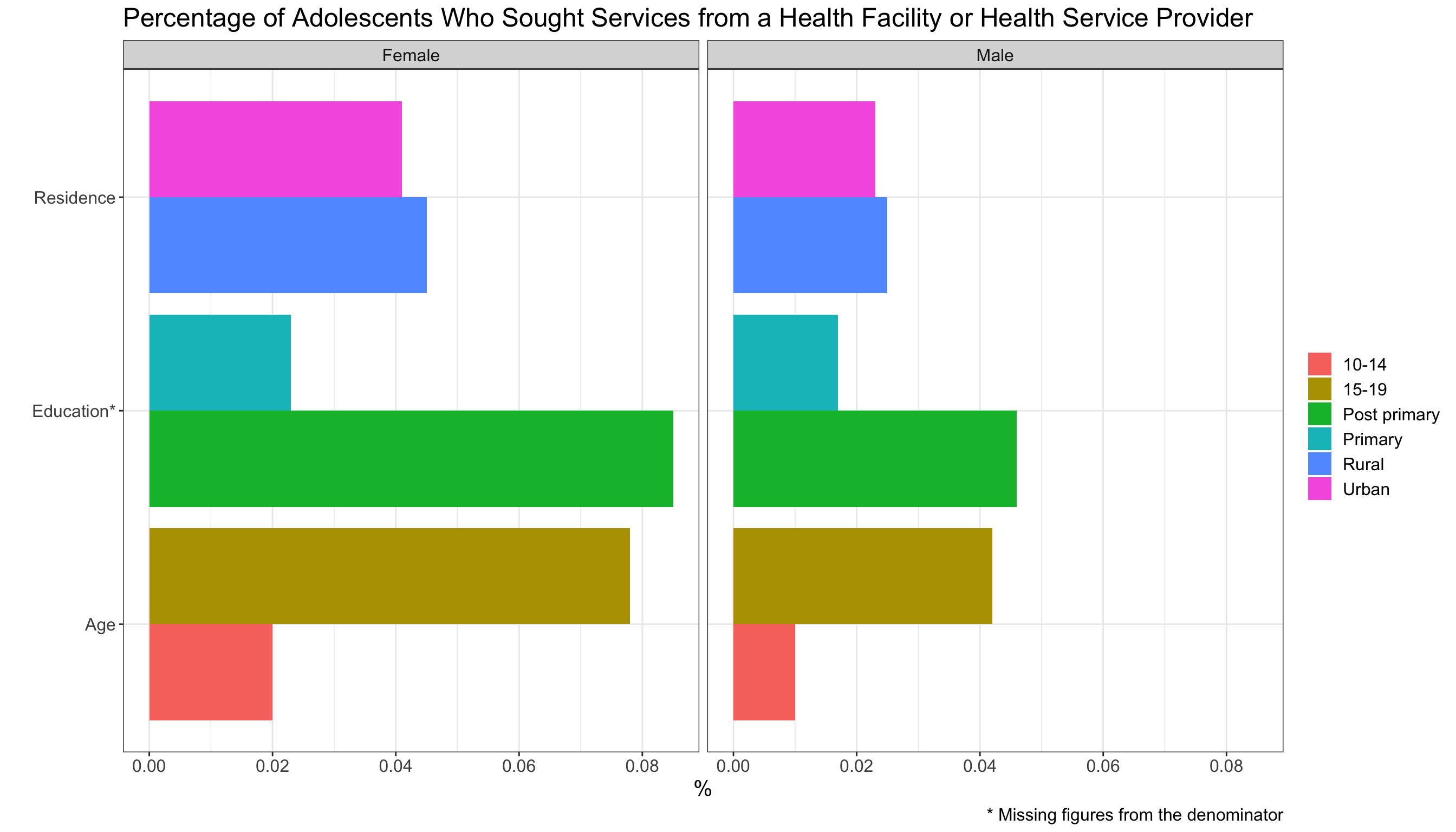
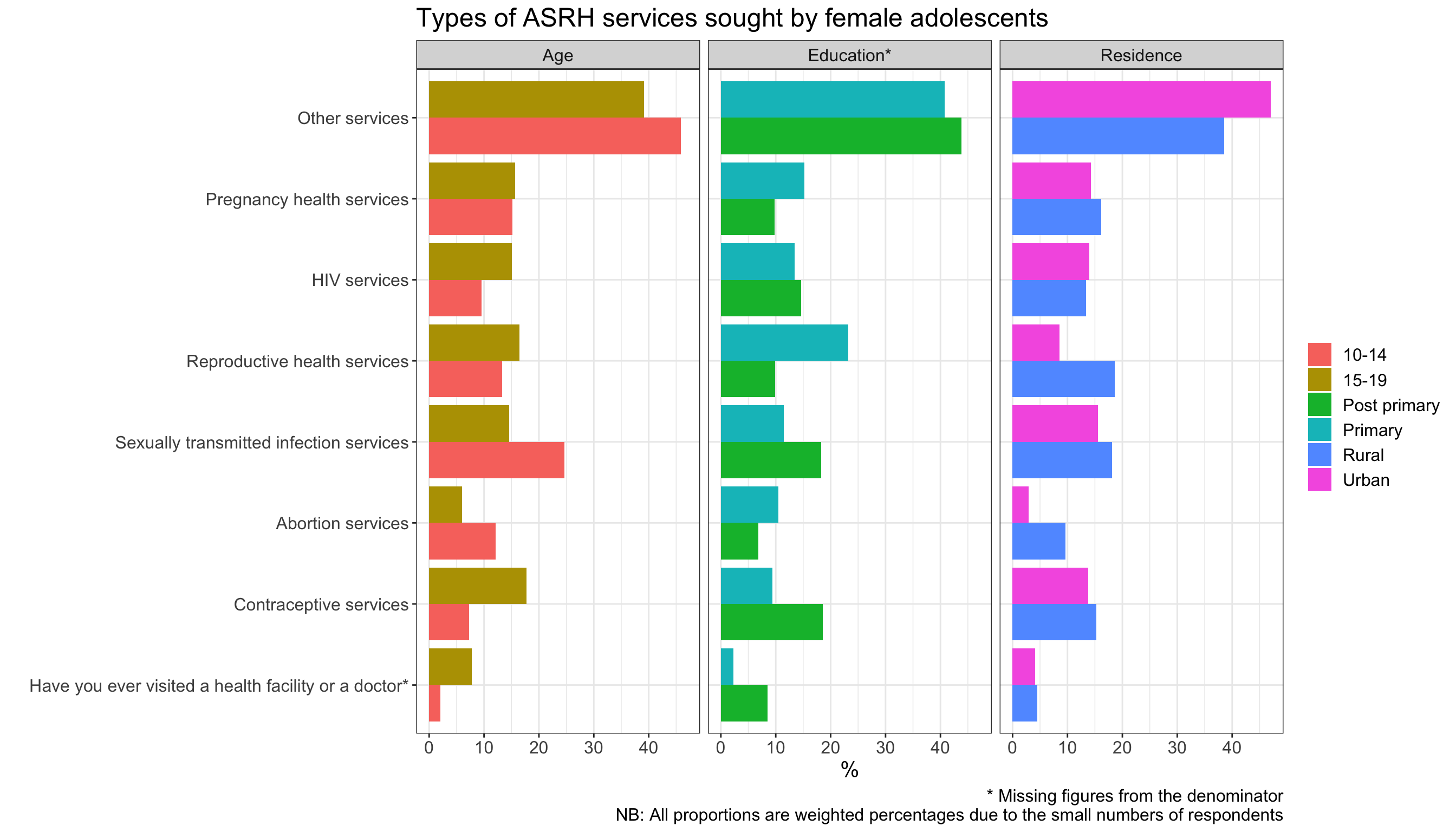
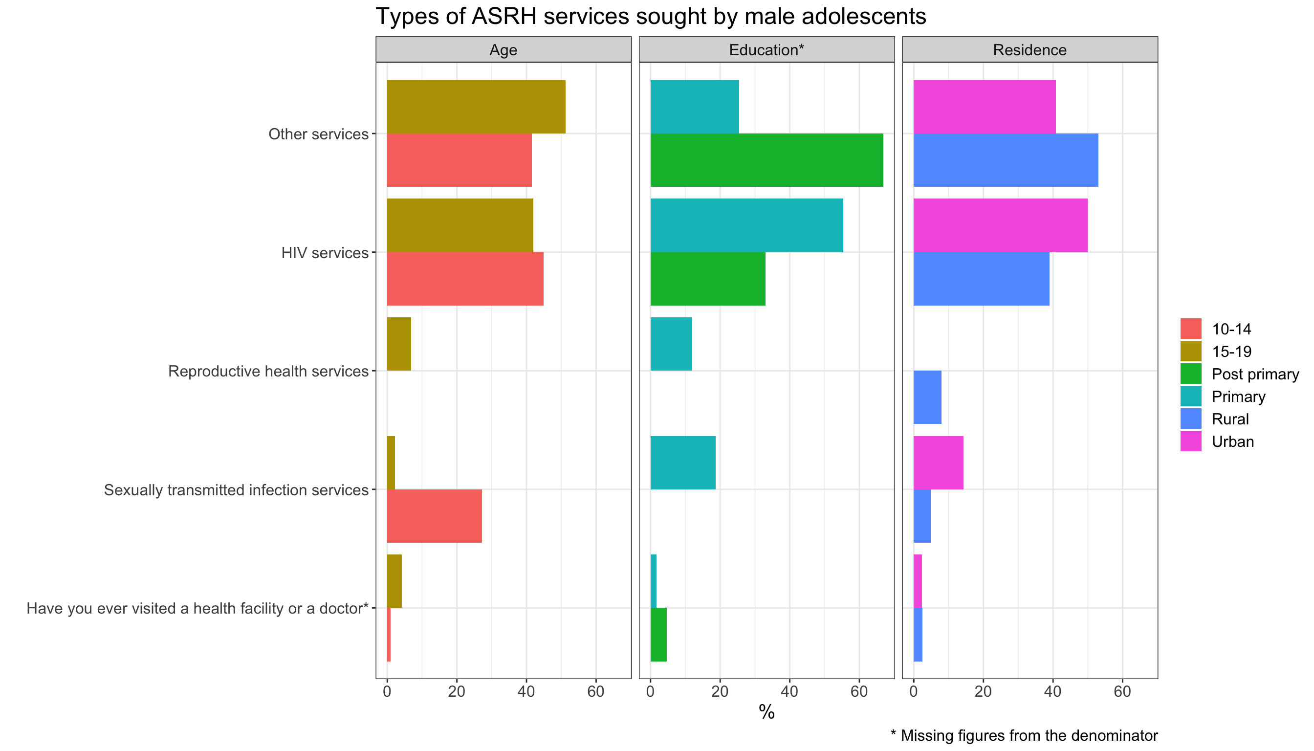
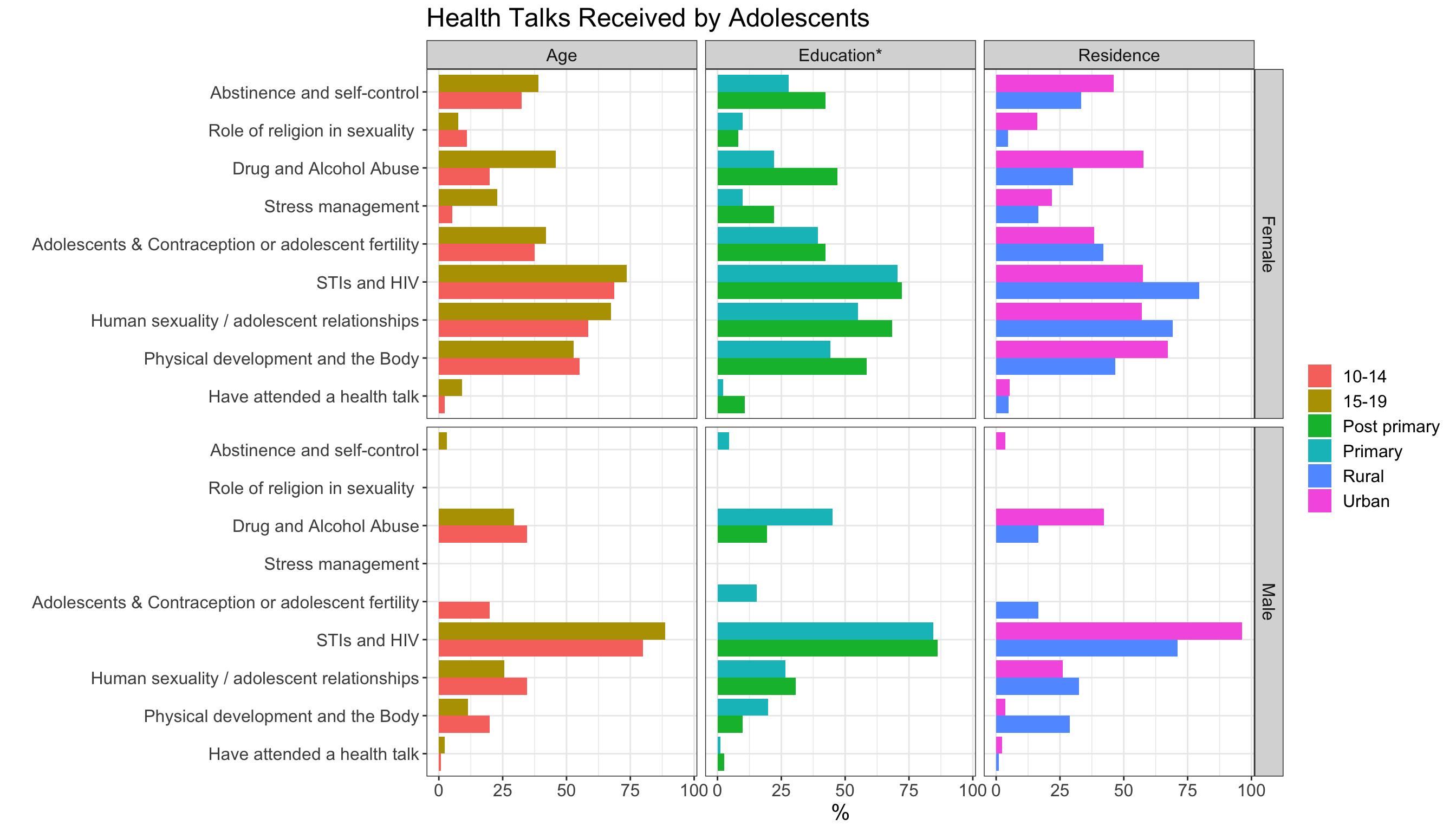
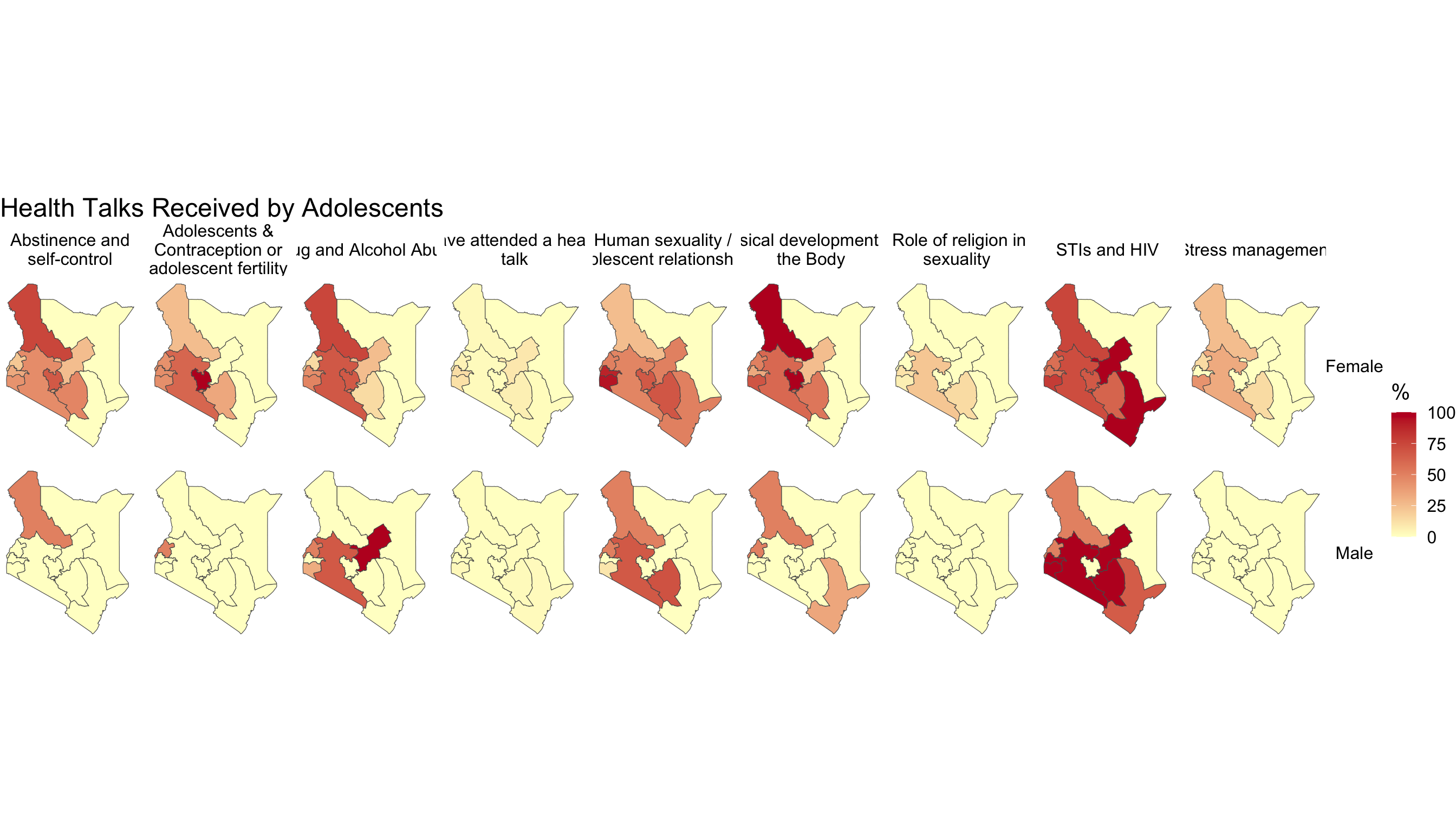

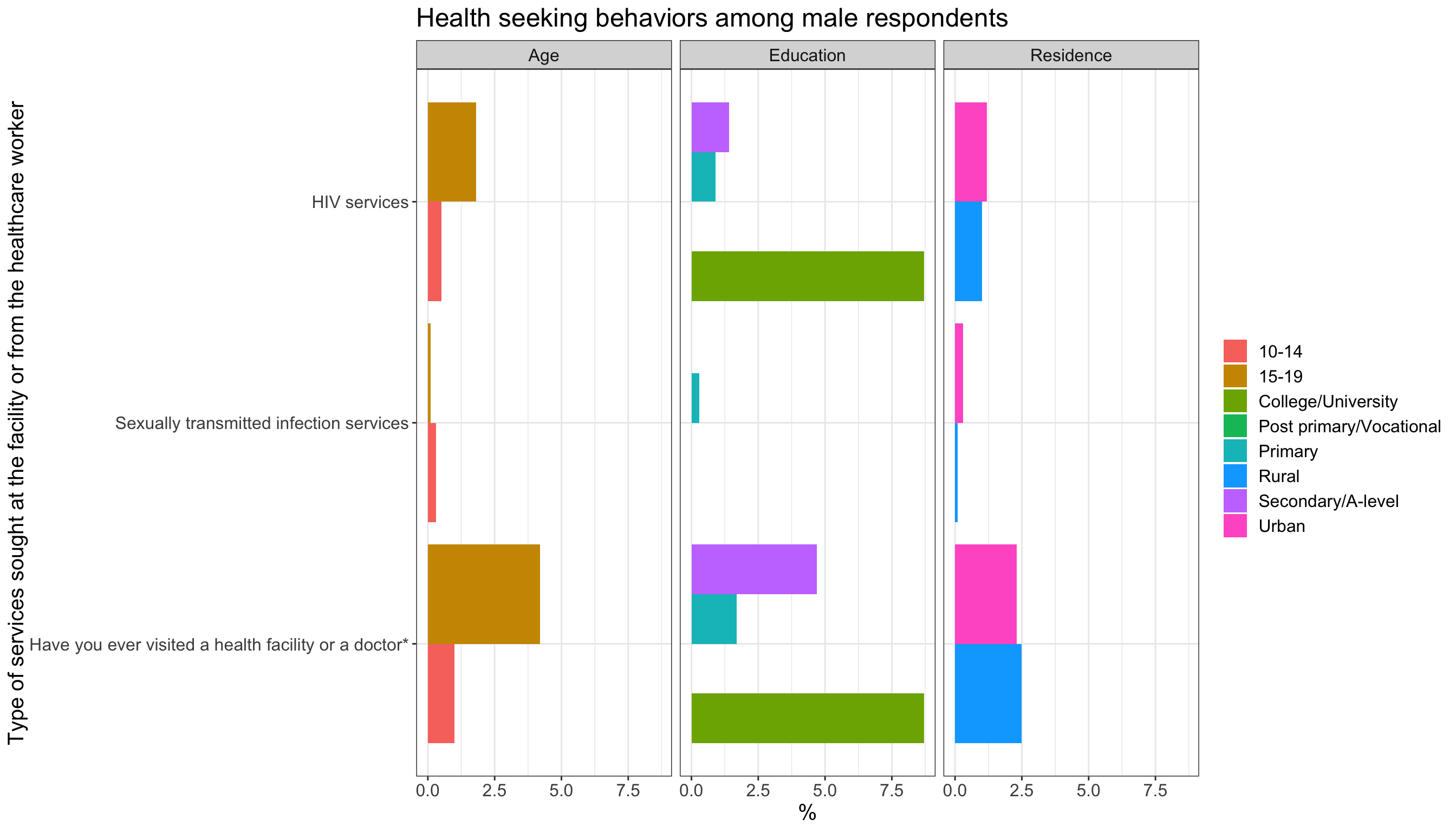


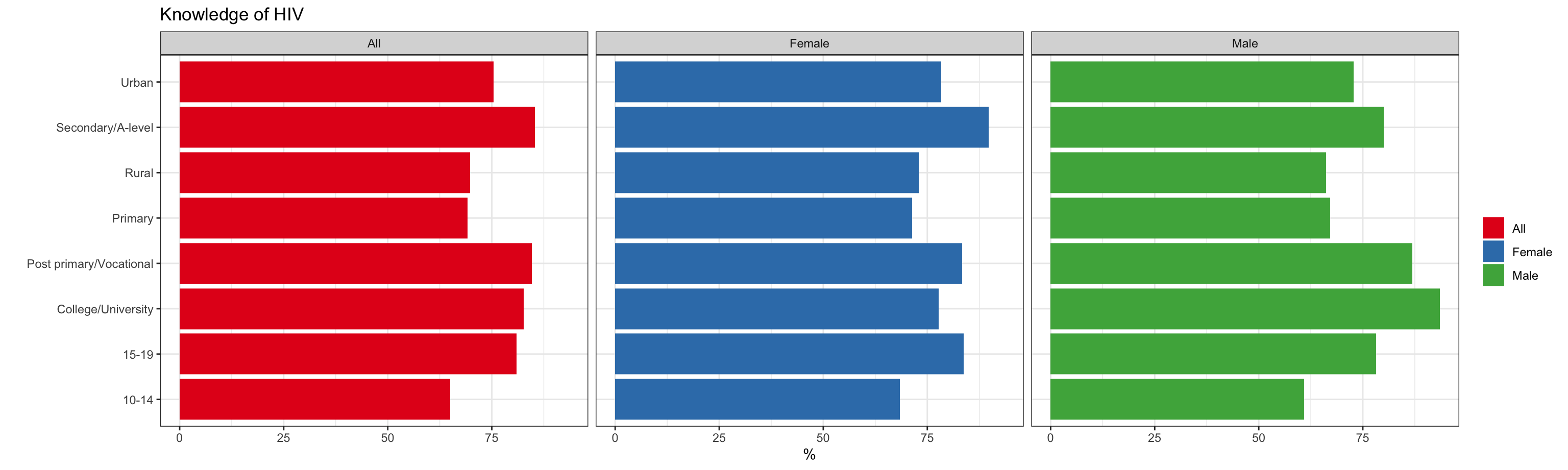

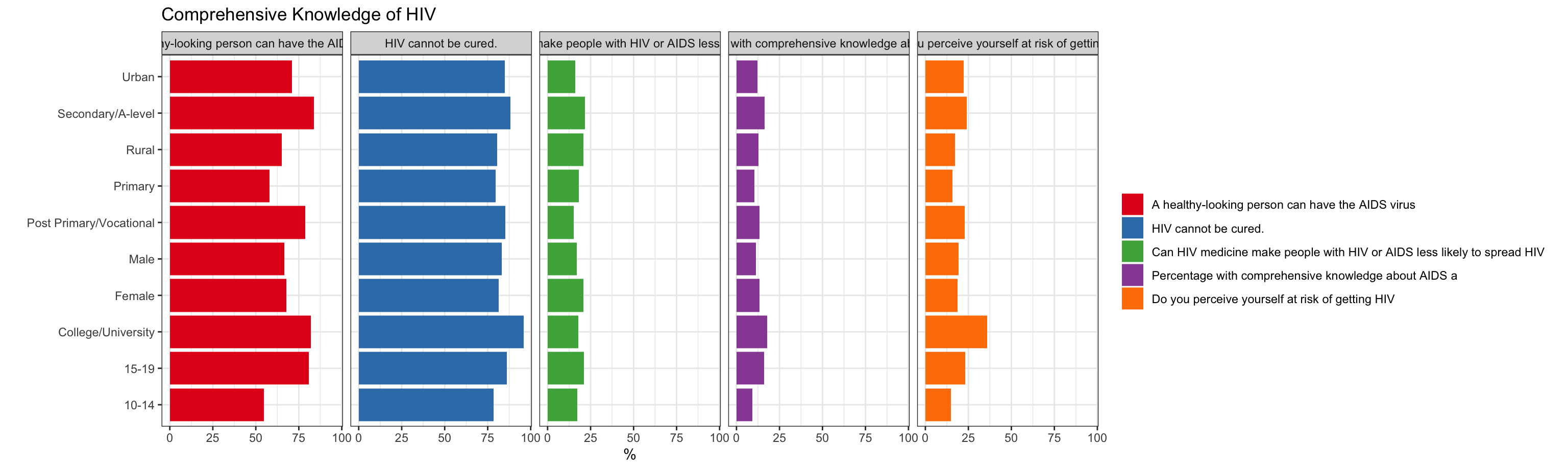

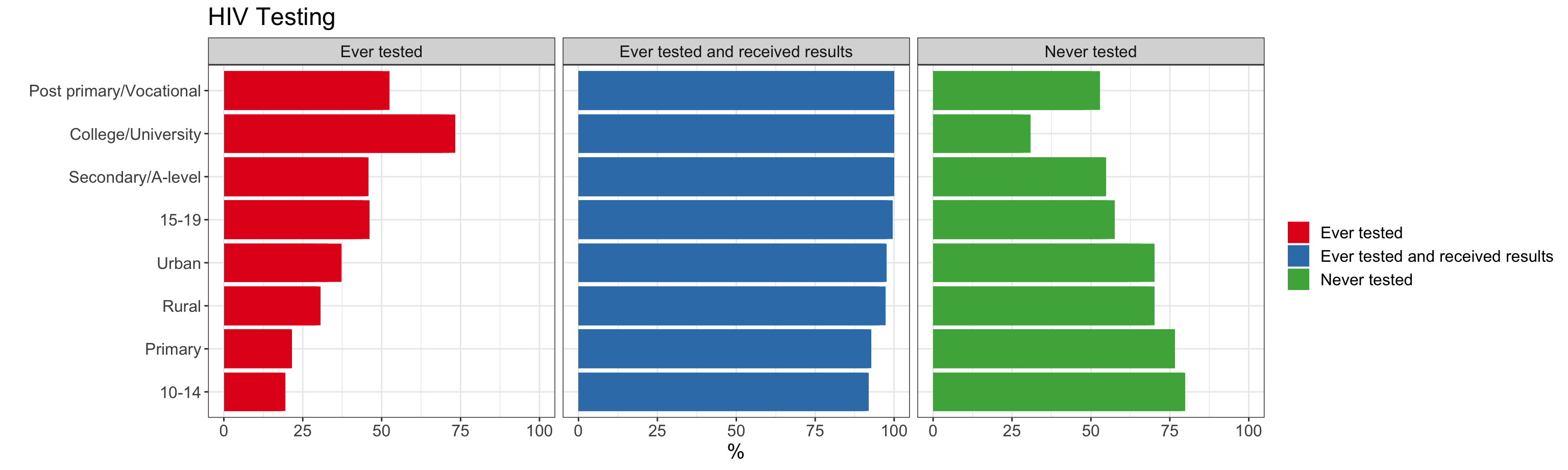

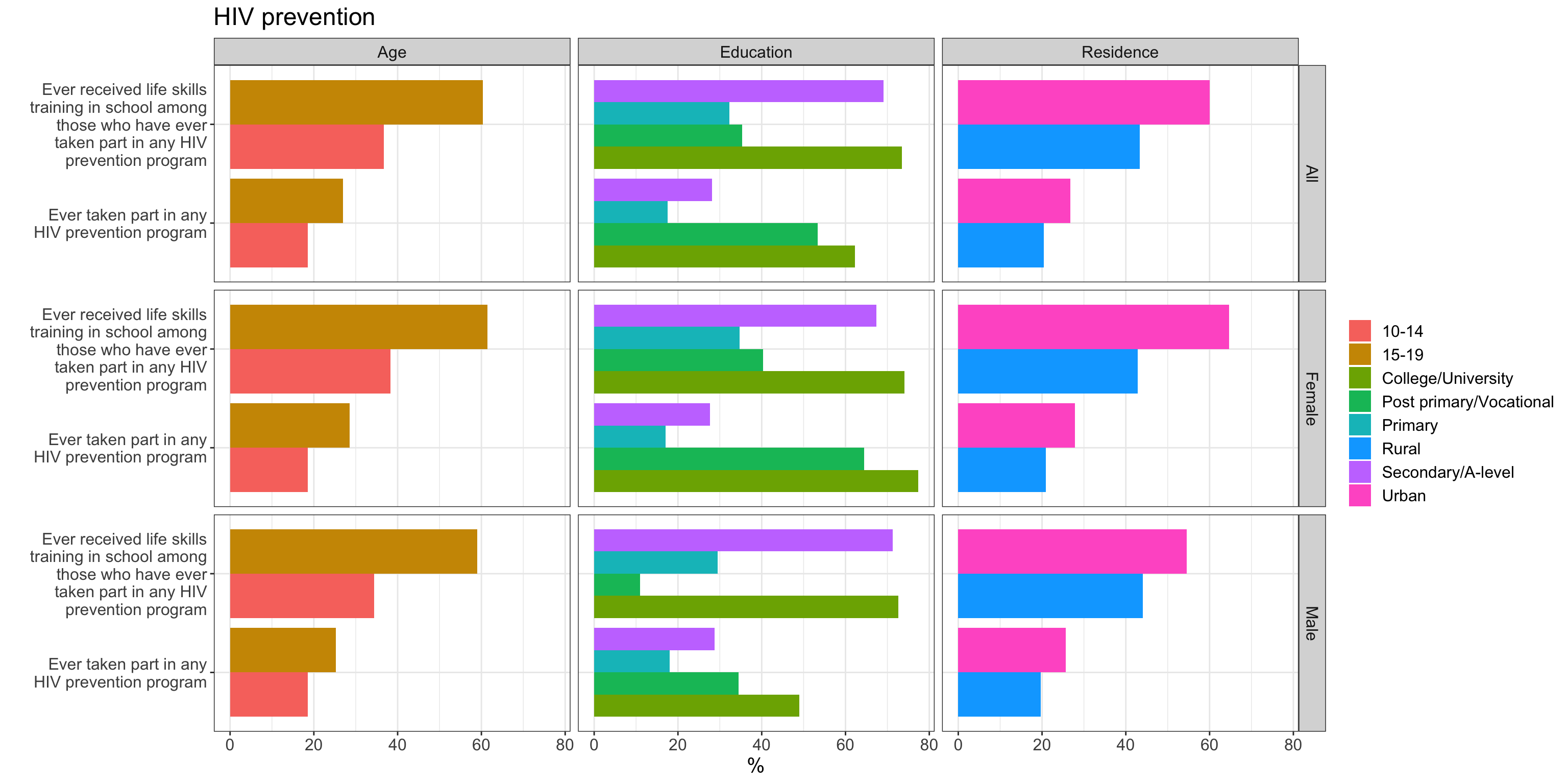
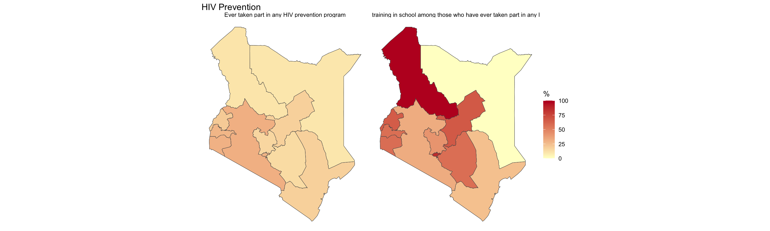
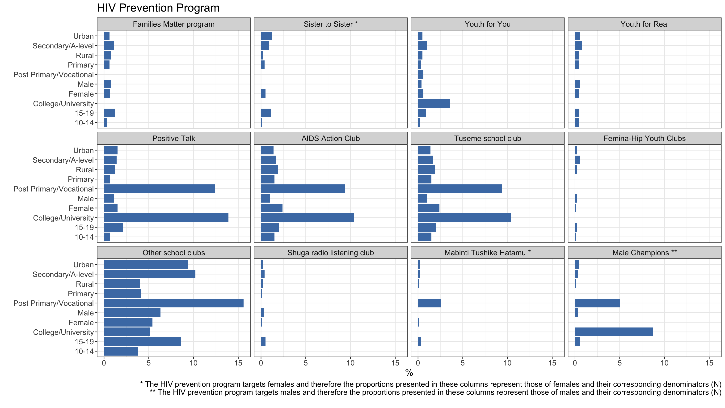

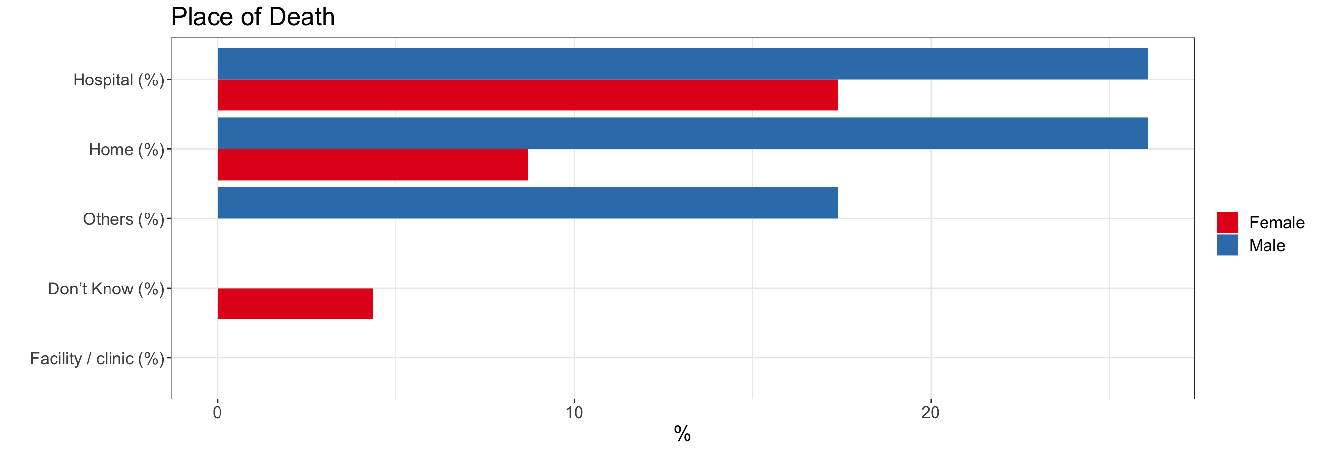
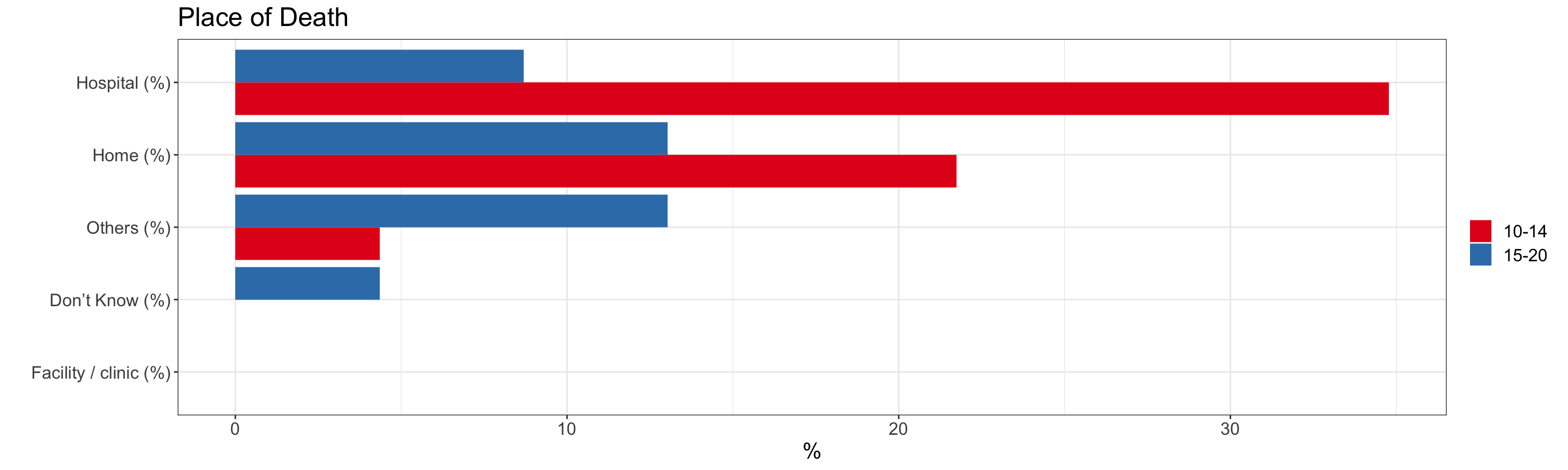
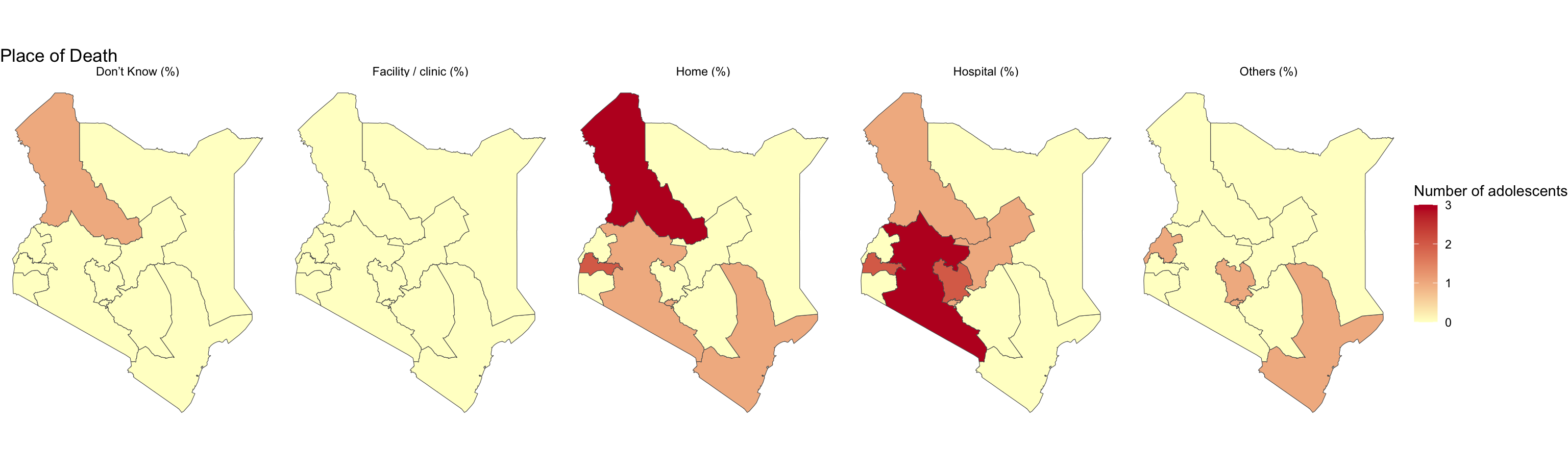
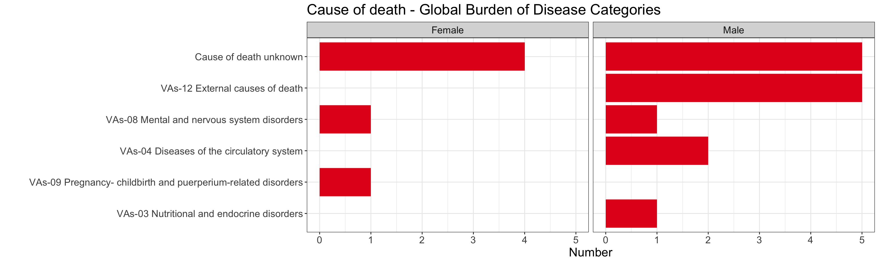


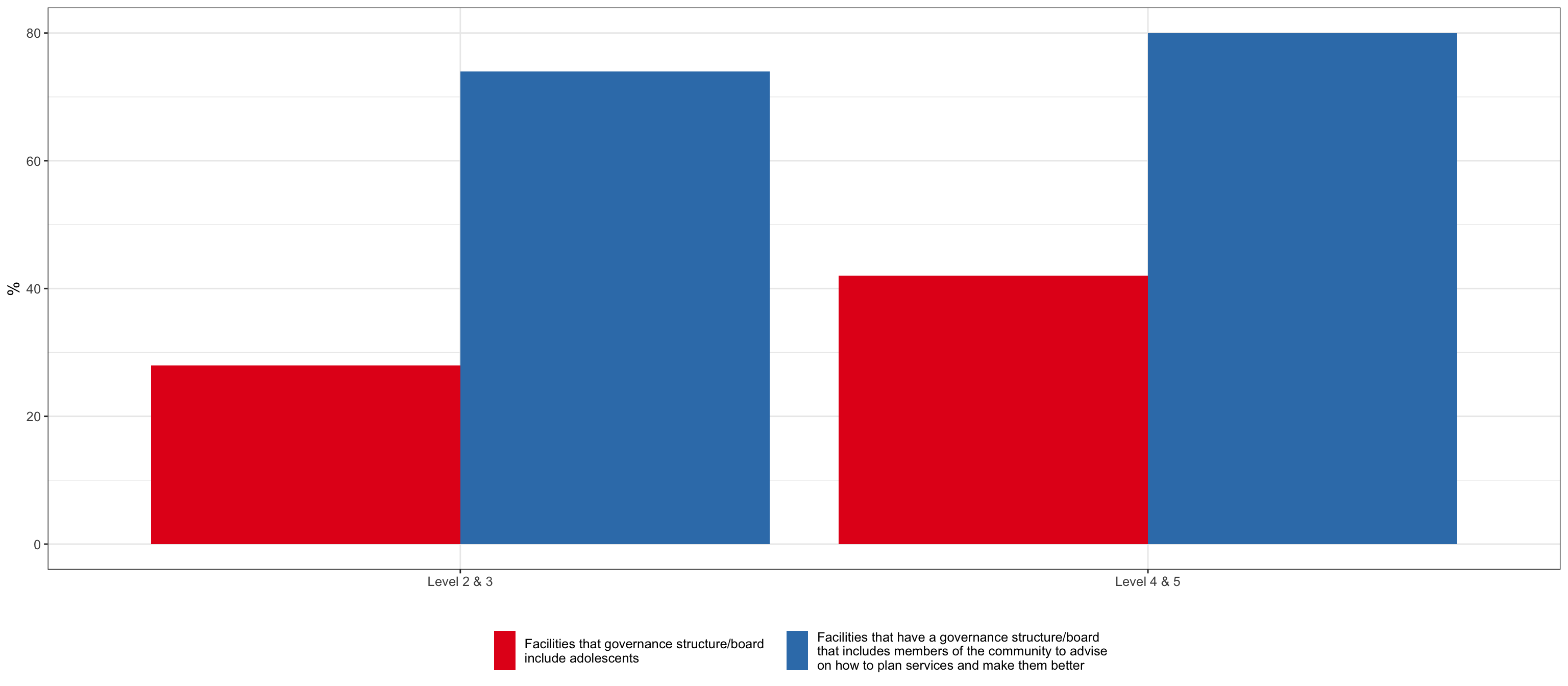
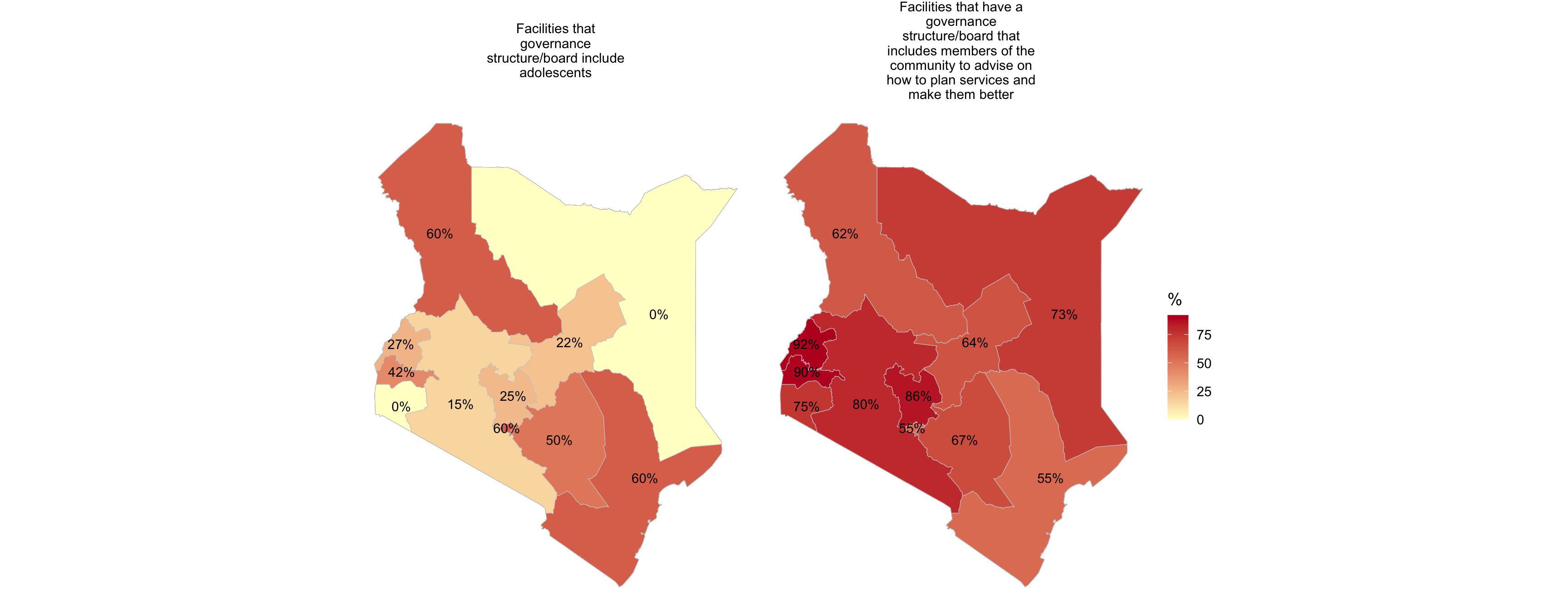
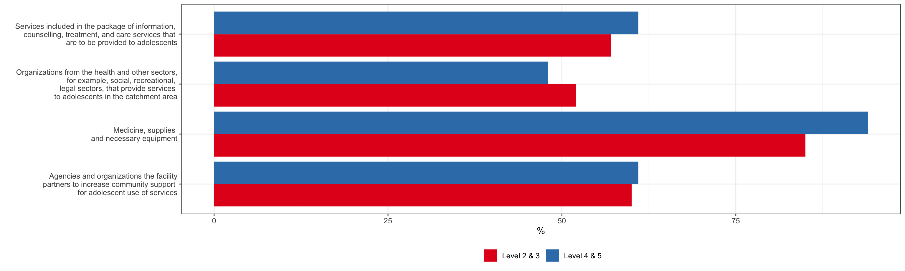
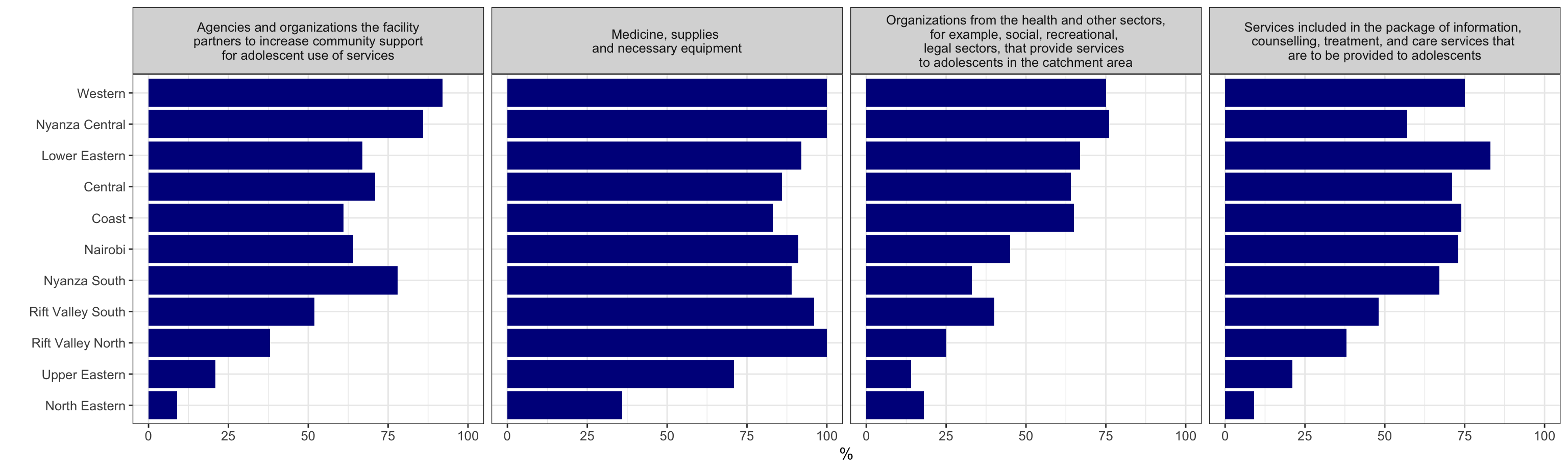


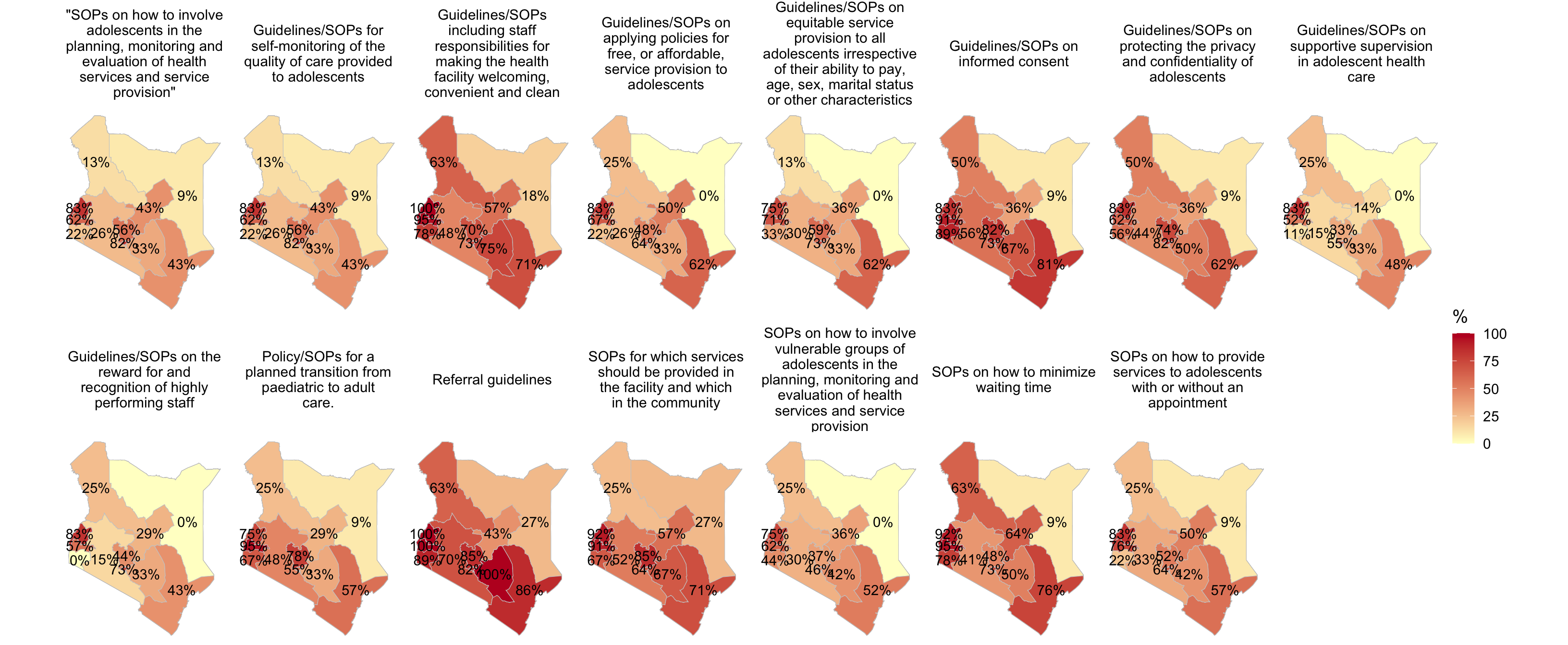
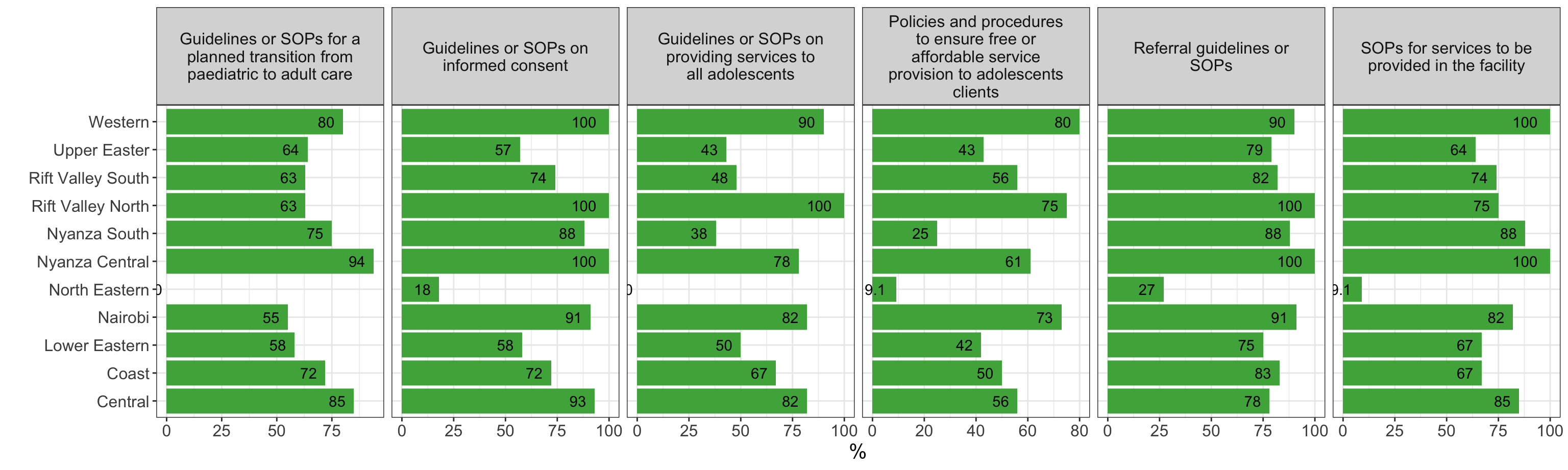


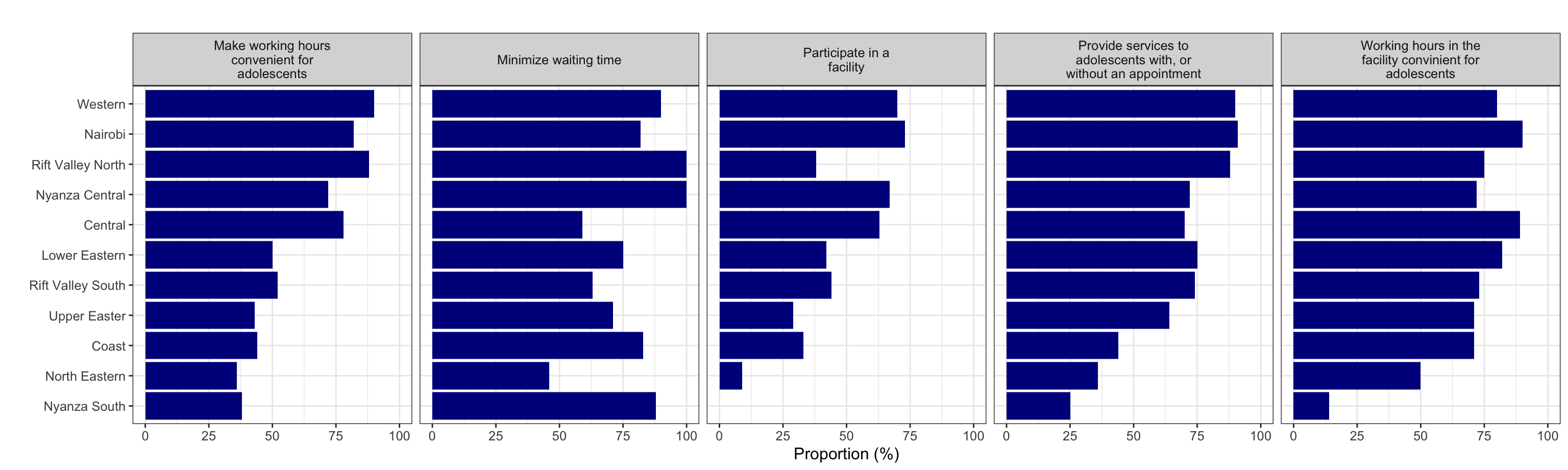
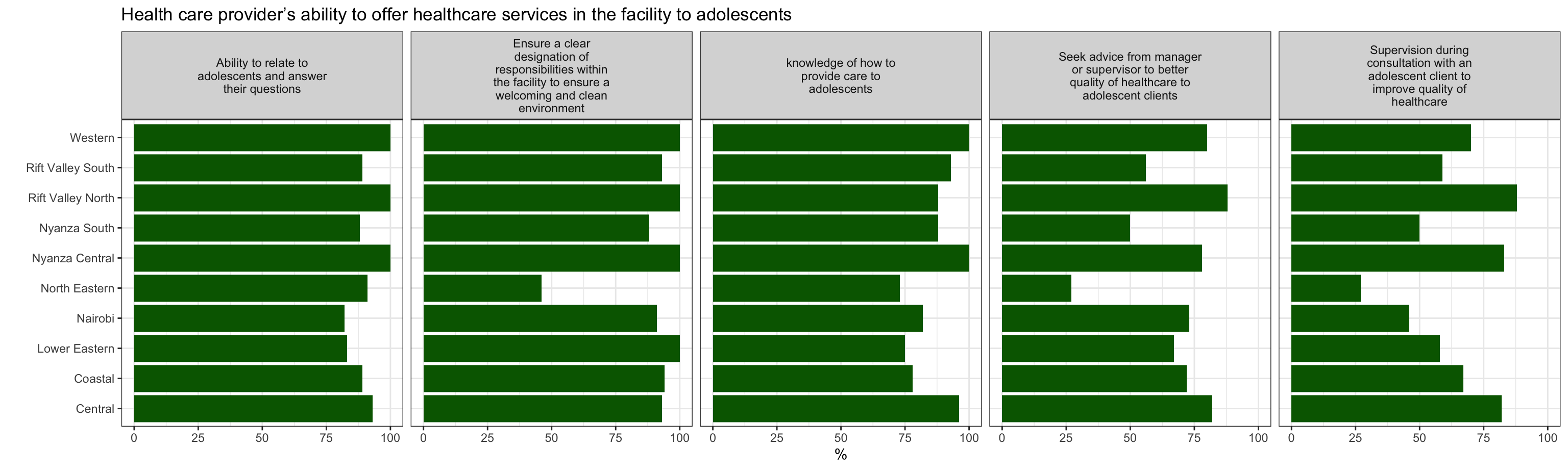
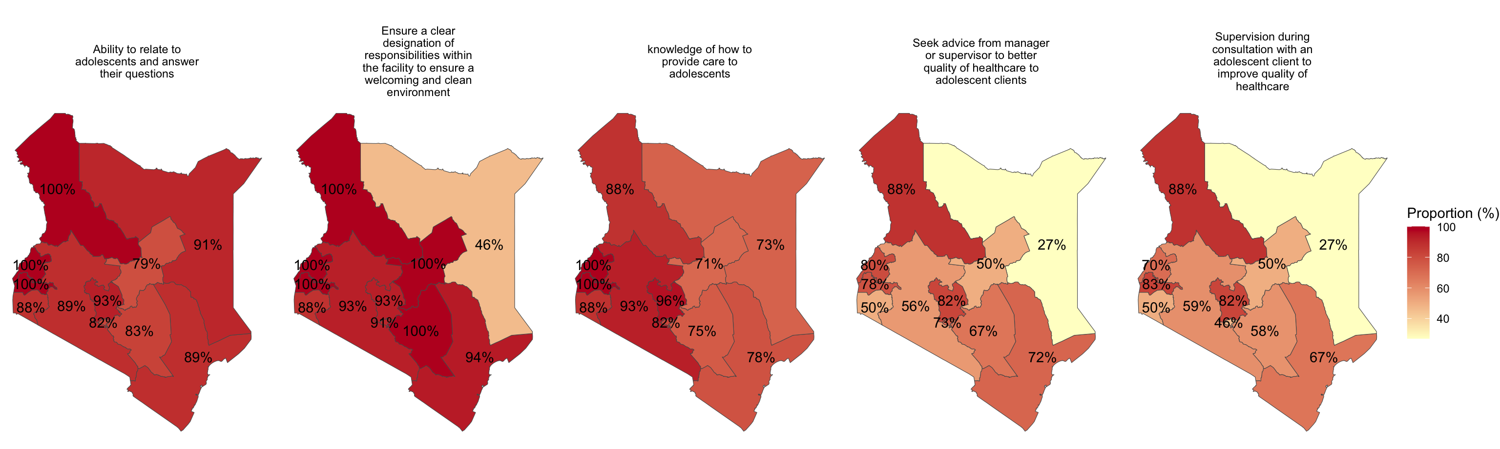
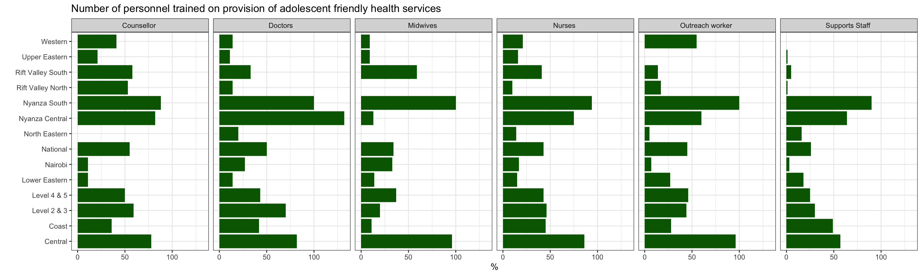
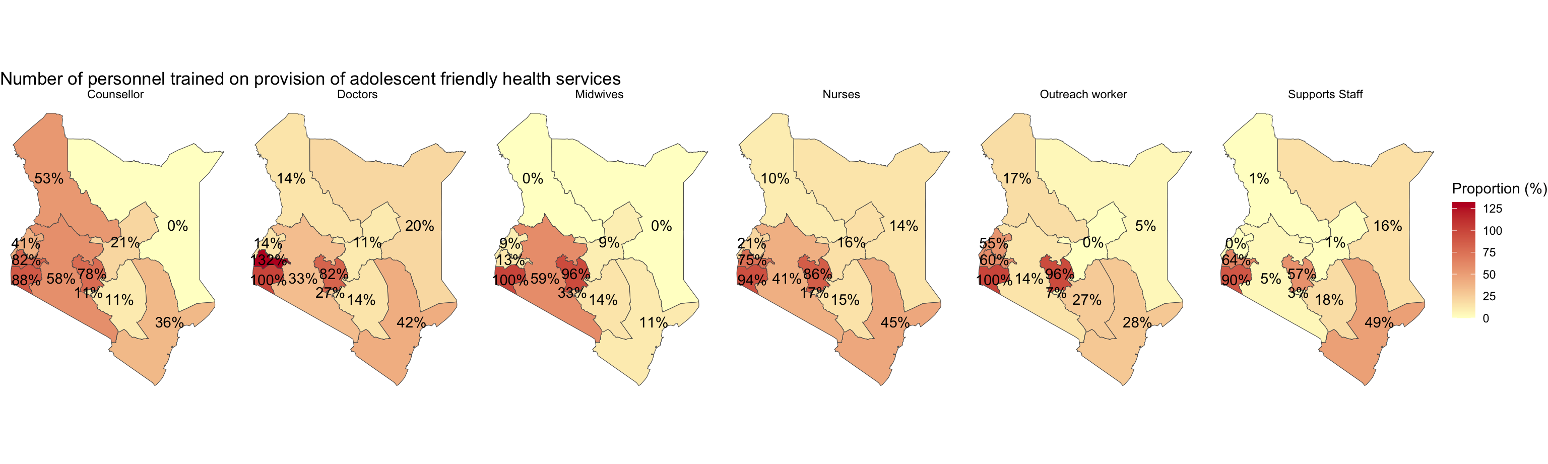
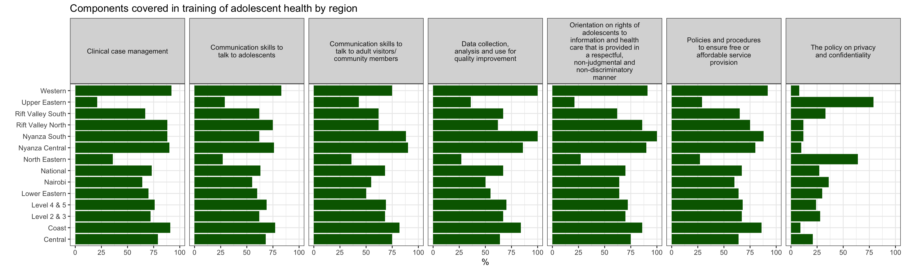
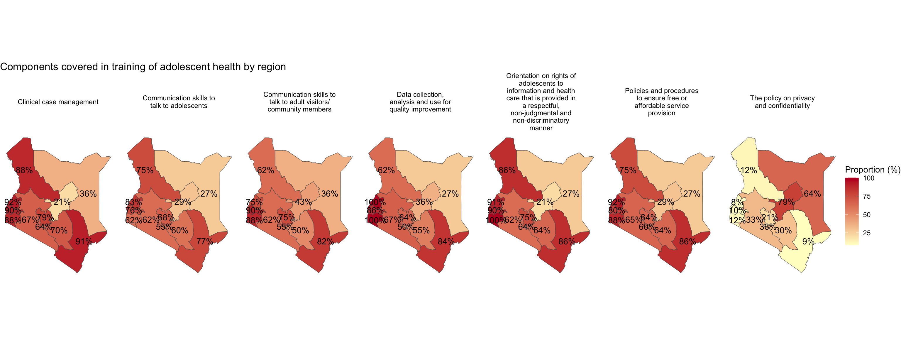
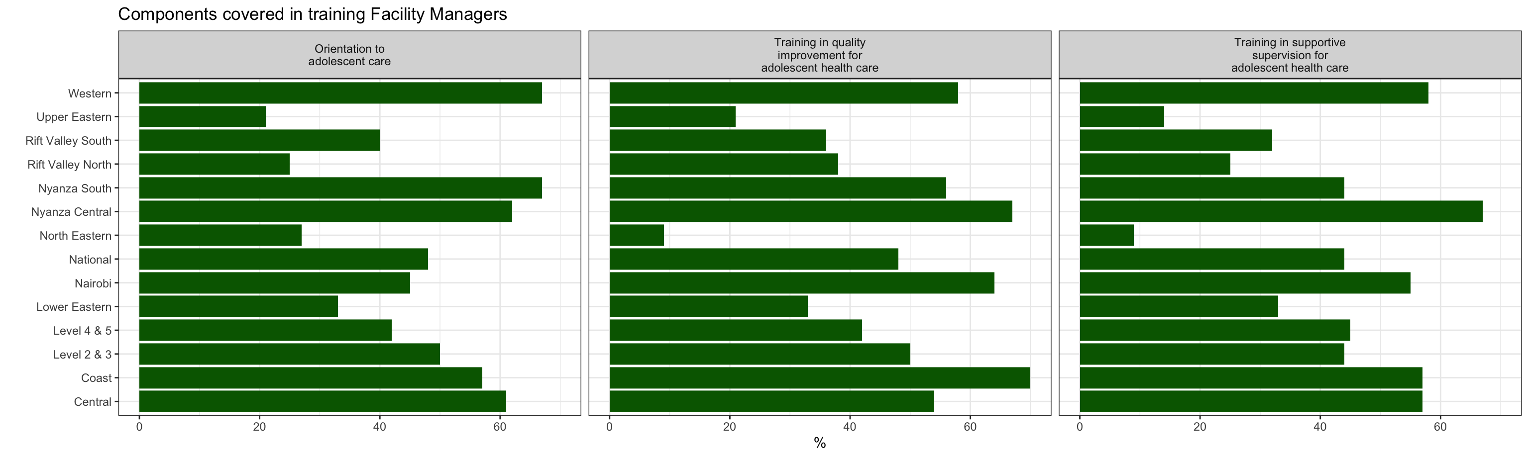
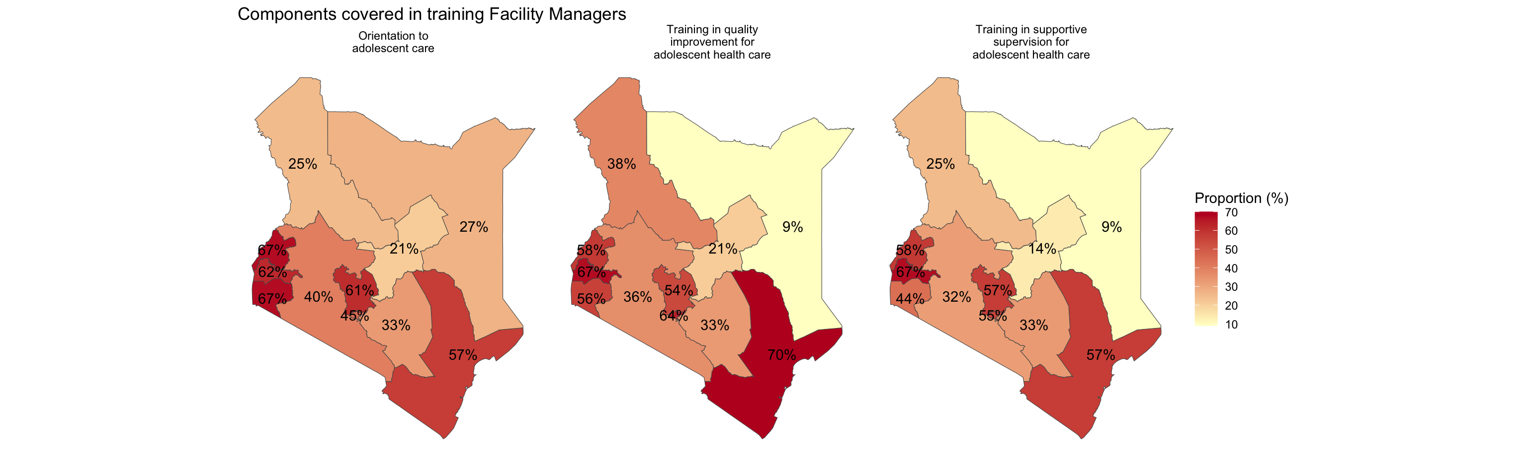
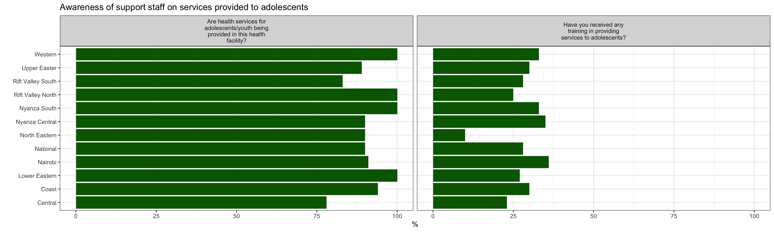
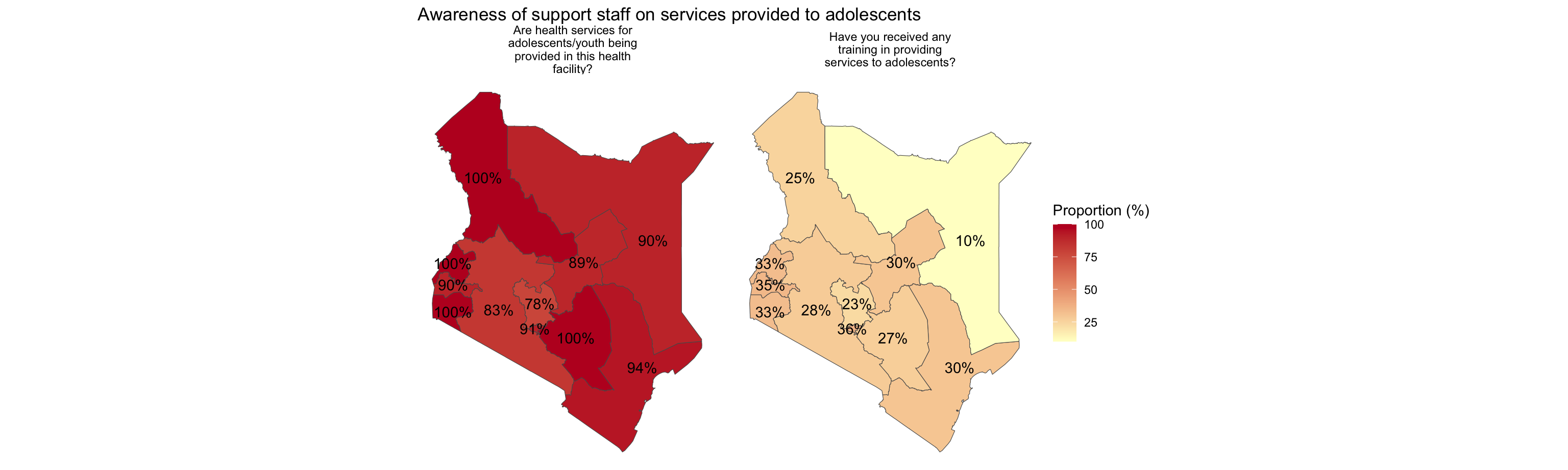
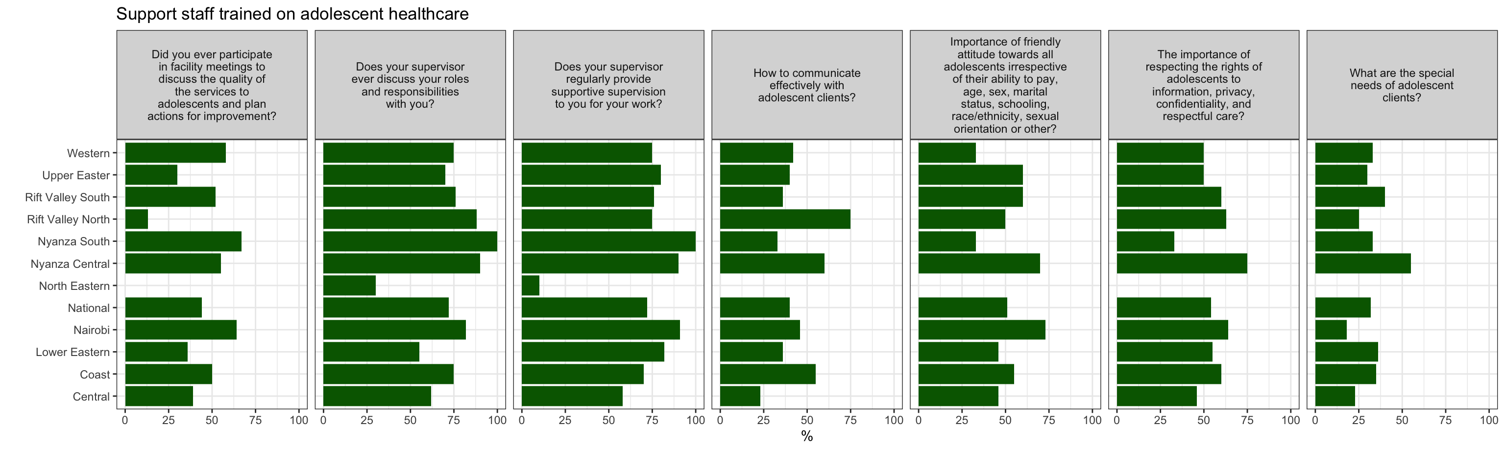


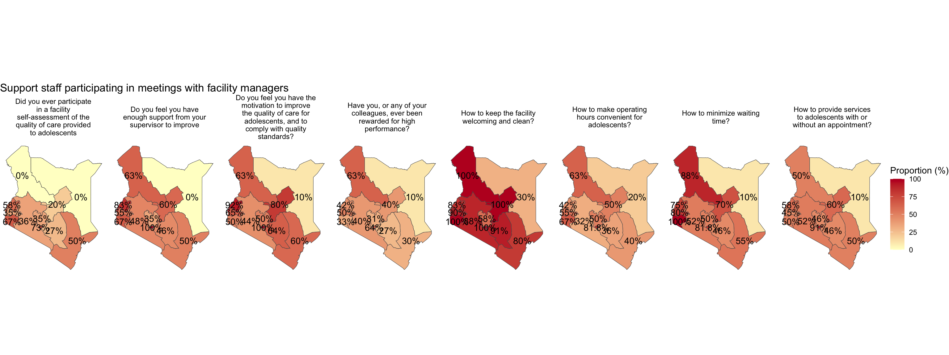
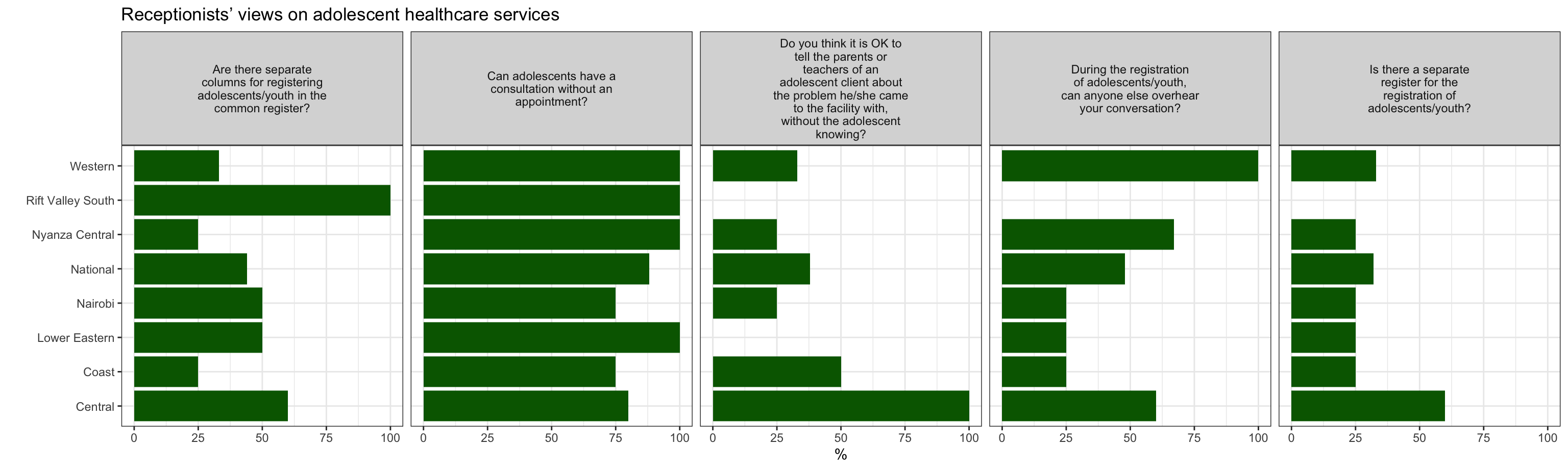
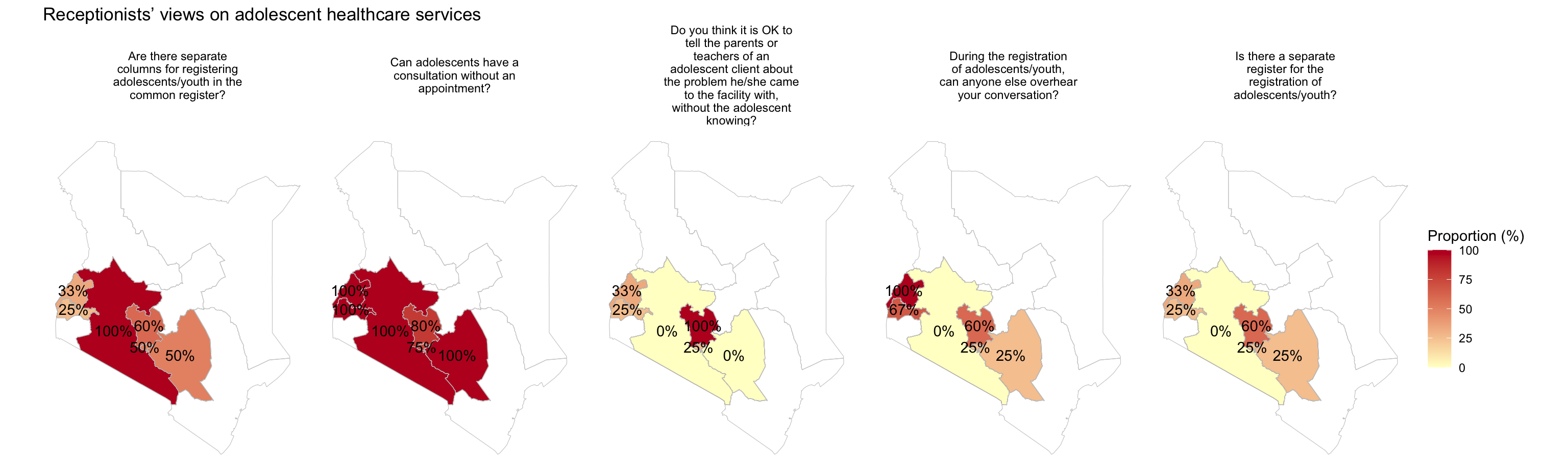
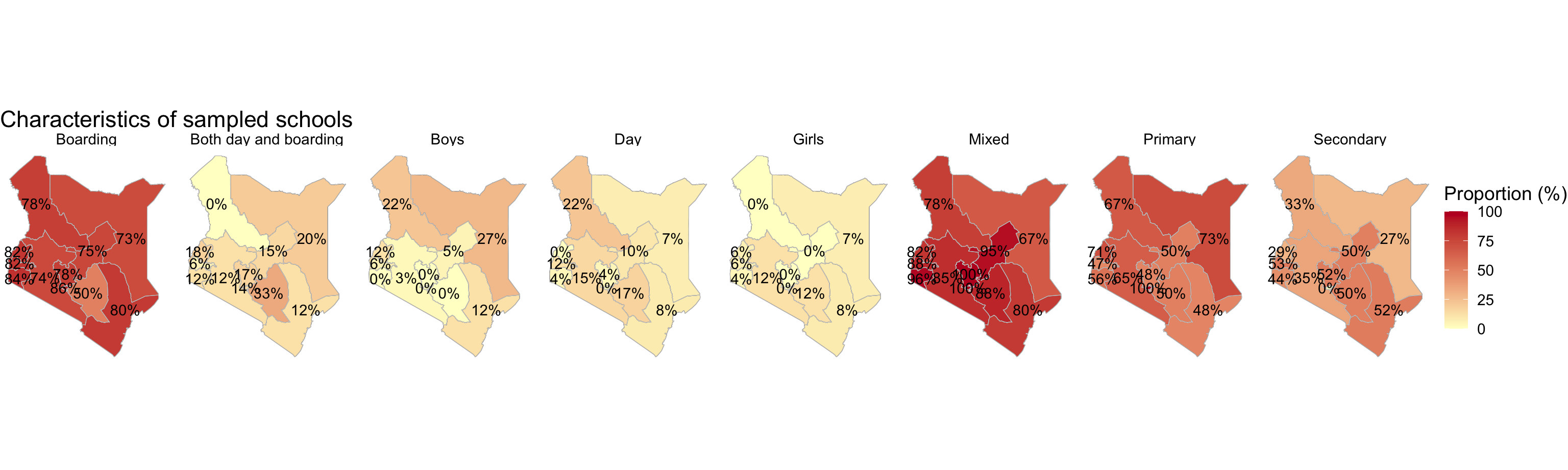
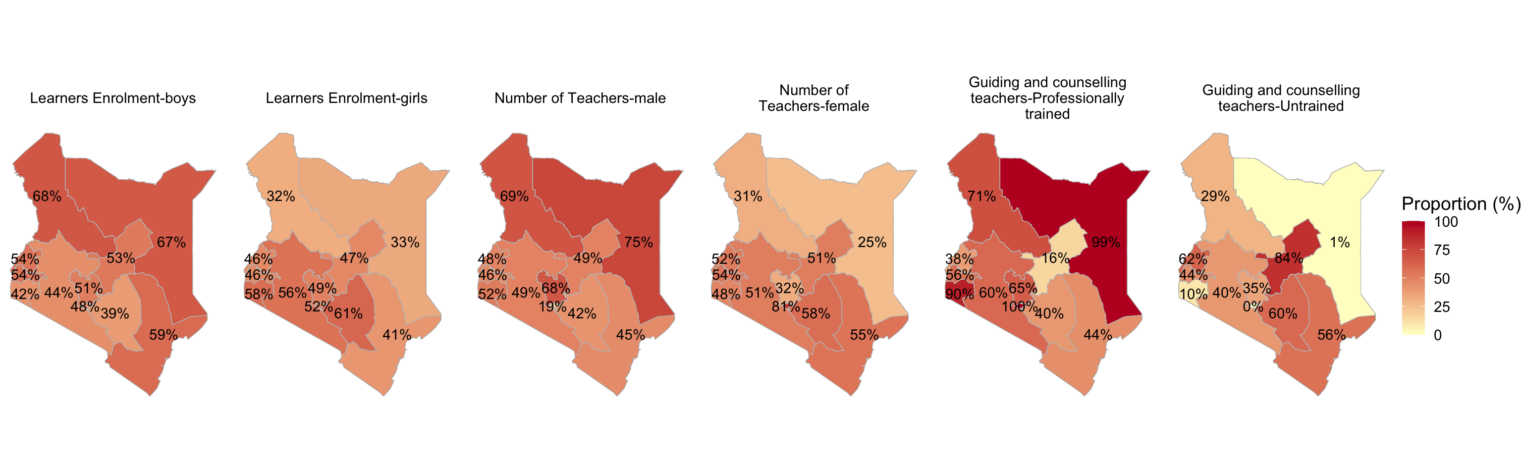
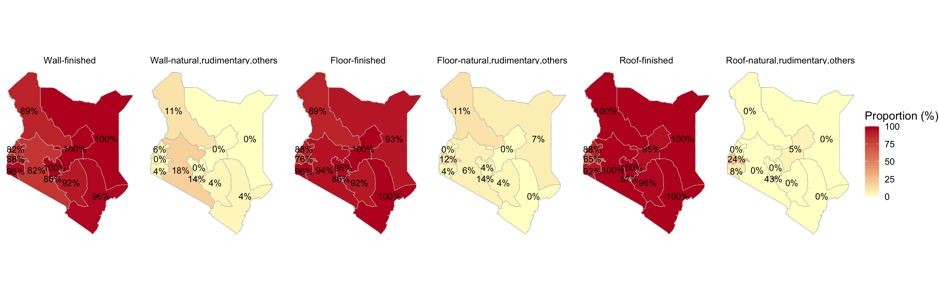
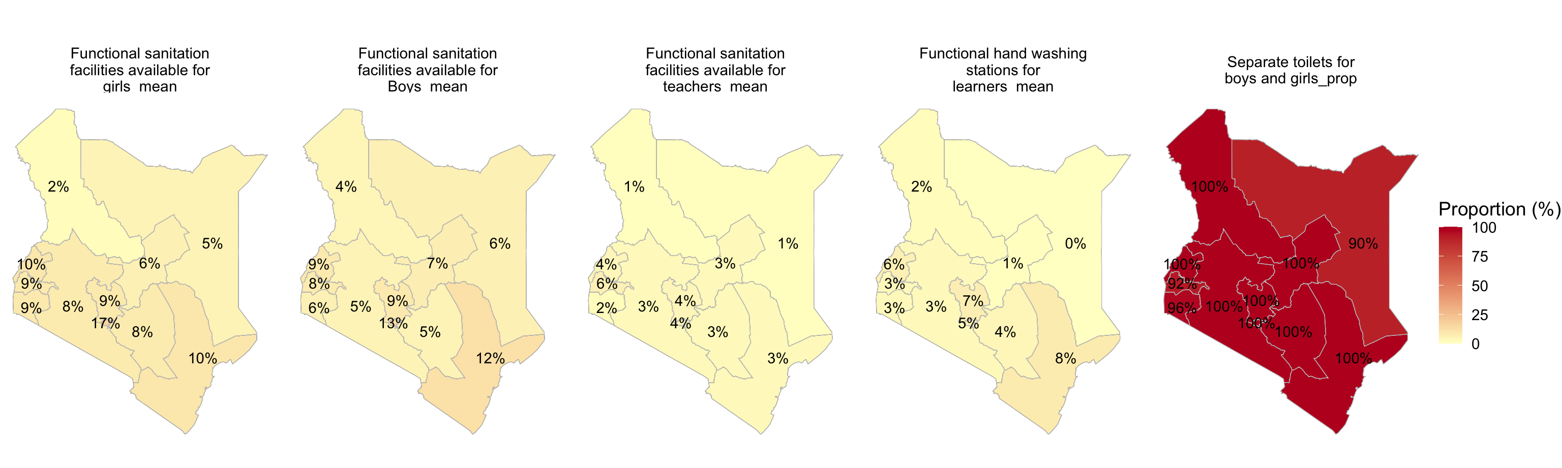
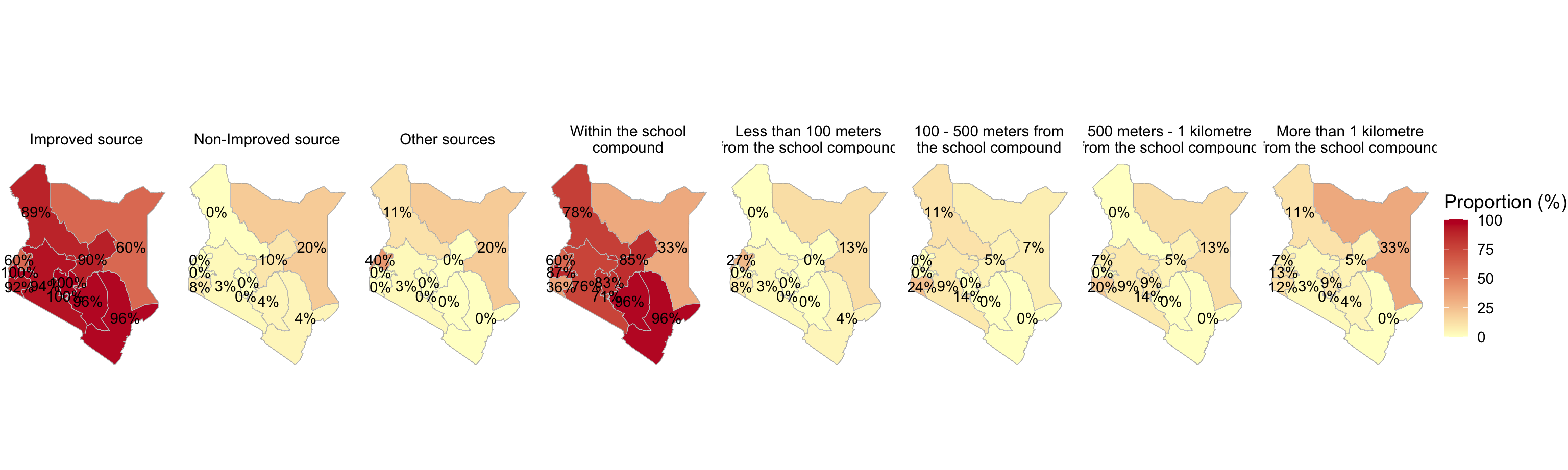
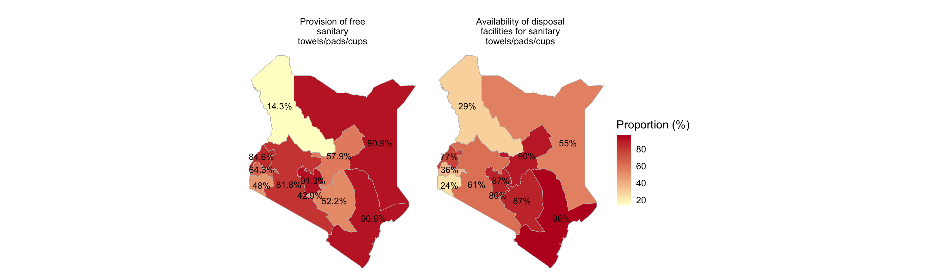
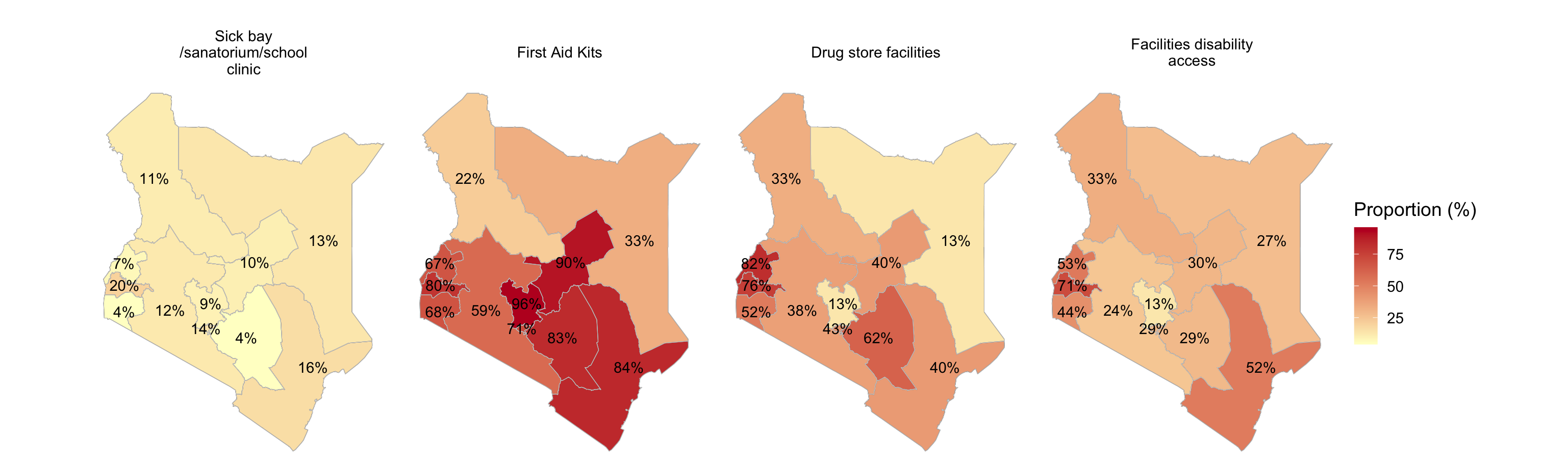

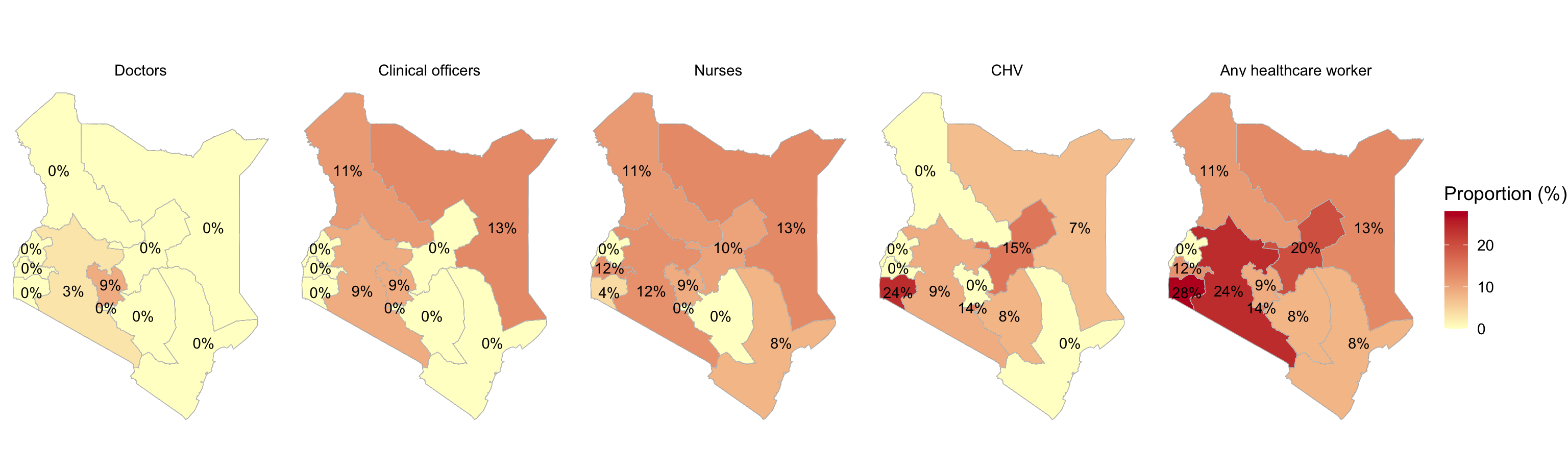

social_characteristics
Inputs
Summary
Household characteristics
Social Demographic characteristics
Social characteristics
Adolescent Nutrition
Physical Activity
Adolescents Mental Health Status
General Adolescent Morbidity
Oral Health
Injuries
Child Functioning/Disability
Adolescent Sexual & Reproductive Health
Adolescent HIV
Adolescent Mortality
Row
ValueBox
ValueBox
ValueBox
Row
Male Essential Expenditure
Female Essential Expenditure
Row
Male Non Essential Expenditure
Female Non-Essential Expenditure